Chapter 1 Introduction to R
R is a computer programming language that was purpose-built for statistical data analysis. The name “R” is a play on the names of the two authors of the software package (Ross Ihaka and Robert Gentleman) as well as an homage to an older statistical software package called “S”. R has become one of the most popular programming languages for statistical analysis and “data science”, which refers to the broader enterprise of working with and analyzing data. Unlike general-purpose programming languages such as Python or Java, R is purpose-built for statistics. That doesn’t mean that you can’t do more general things with it, but the place where it really shines is in data analysis and statistics.
1.1 Why programming is hard to learn
Programming a computer is a skill, just like playing a musical instrument or speaking a second language. And just like those skills, it takes a lot of work to get good at it — the only way to acquire a skill is through practice. There is nothing special or magical about people who are experts, other than the quality and quantity of their experience! However, not all practice is equally effective. A large amount of psychological research has shown that practice needs to be deliberate, meaning that it focuses on developing the specific skills that one needs to perform the activity, at a level that is always pushing one’s ability.
If you have never programmed before, then it’s going to seem hard, just as it would seem hard for a native English speaker to start speaking Mandarin. However, just as a beginning guitarist needs to learn to play their scales, we will teach you how to perform the basics of programming, which you can then use to do more powerful things.
One of the most important aspects of computer programming is that you can try things to your heart’s content; the worst thing that can happen is that the program will crash. Trying new things and making mistakes is one of the keys to learning.
The hardest part of programming is figuring out why something didn’t work, which we call debugging. In programming, things are going to go wrong in ways that are often confusing and opaque. Every programmer has a story about spending hours trying to figure out why something didn’t work, only to realize that the problem was completely obvious. The more practice you get, the better you will get at figuring out how to fix these errors. But there are a few strategies that can be helpful.
1.1.1 Use the web
In particular, you should take advantage of the fact that there are millions of people programming in R around the world, so nearly any error message you see has already been seen by someone else. Whenever I experience an error that I don’t understand, the first thing that I do is to copy and paste the error message into a search engine. Often this will provide several links discussing the problem and the ways that people have solved it.
1.2 Using RStudio
When I am using R in my own work, I generally use a free software package called RStudio, which provides a number of nice tools for working with R. In particular, RStudio provides the ability to create “notebooks” that mix together R code and text (formatted using the Markdown text formatting system). In fact, this book is written using exactly that system! You can see the R code used to generate this book here.
In some cases it m ay not be possible to install RStudio on one’s computer (for example, if that computer is a Chromebook). Another alteranative is to use an online platform for coding. Two popular platforms that support R are Google’s Colab and Kaggle Kernels.
1.3 Getting started with R
When we work with R, we often do this using a command line in which we type commands and it responds to those commands. In the simplest case, if we just type in a number, it will simply respond with that number. Go into the R console and type the number 3. You should see something like this:
> 3
[1] 3
The > symbol is the command prompt, which is prompting you to type something in. The next line ([1] 3) is R’s answer. Let’s try something a bit more complicated:
> 3 + 4
[1] 7
R spits out the answer to whatever you type in, as long as it can figure it out. Now let’s try typing in a word:
> hello
Error: object 'hello' not found
What? Why did this happen? When R encounters a letter or word, it assumes that it is referring to the name of a variable — think of X from high school algebra. We will return to variables in a little while, but if we want R to print out the word hello then we need to contain it in quotation marks, telling R that it is a character string.
> "hello"
[1] "hello"
There are many types of variables in R. You have already seen two examples: integers (like the number 3) and character strings (like the word “hello”). Another important one is real numbers, which are the most common kind of numbers that we will deal with in statistics, which span the entire number line including the spaces in between the integers. For example:
> 1/3
[1] 0.33
In reality the result should be 0.33 followed by an infinite number of threes, but R only shows us two decimal points in this example.
Another kind of variable is known as a logical variable, because it is based on the idea from logic that a statement can be either true or false. In R, these are capitalized (TRUE and FALSE).
To determine whether a statement is true or not, we use logical operators. You are already familiar with some of these, like the greater-than (>) and less-than (<) operators.
> 1 < 3
[1] TRUE
> 2 > 4
[1] FALSE
Often we want to know whether two numbers are equal or not equal to one another. There are special operators in R to do this: == for equals, and != for not-equals:
> 3 == 3
[1] TRUE
> 4 != 4
[1] FALSE
1.4 Variables
A variable is a symbol that stands for another value (just like “X” in algebra). We can create a variable by assigning a value to it using the <- operator. If we then type the name of the variable R will print out its value.
> x <- 4
> x
[1] 4
The variable now stands for the value that it contains, so we can perform operations on it and get the same answer as if we used the value itself.
> x + 3
[1] 7
> x == 5
[1] FALSE
We can change the value of a variable by simply assigning a new value to it.
> x <- x + 1
> x
[1] 5
A note: You can also use the equals sign = instead of the <-
1.5 Functions
A function is an operator that takes some input and gives an output based on the input. For example, let’s say that we have a number, and we want to determine its absolute value. R has a function called abs() that takes in a number and outputs its absolute value:
> x <- -3
> abs(x)
[1] 3
Most functions take an input like the abs() function (which we call an argument), but some also have special keywords that can be used to change how the function works. For example, the rnorm() function generates random numbers from a normal distribution (which we will learn more about later). Have a look at the help page for this function by typing help(rnorm) in the console, which will cause a help page to appear below. The section of the help page for the rnorm() function shows the following:
rnorm(n, mean = 0, sd = 1)

Arguments

n     number of observations.

mean    vector of means.

sd   vector of standard deviations.
You can also obtain some examples of how the function is used by typing example(rnorm) in the console.
We can see that the rnorm function has two arguments, mean and sd, that are shown to be equal to specific values. This means that those values are the default settings, so that if you don’t do anything, then the function will return random numbers with a mean of 0 and a standard deviation of 1. The other argument, n, does not have a default value. Try typing in the function rnorm() with no arguments and see what happens — it will return an error telling you that the argument “n” is missing and does not have a default value.
If we wanted to create random numbers with a different mean and standard deviation (say mean == 100 and standard deviation == 15), then we could simply set those values in the function call. Let’s say that we would like 5 random numbers from this distribution:
> my_random_numbers <- rnorm(5, mean=100, sd=15)
> my_random_numbers
[1] 104 115 101  97 115
You will see that I set the variable to the name my_random_numbers. In general, it’s always good to be as descriptive as possible when creating variables; rather than calling them x or y, use names that describe the actual contents. This will make it much easier to understand what’s going on once things get more complicated.
1.6 Vectors
You may have noticed that the my_random_numbers created above wasn’t like the variables that we had seen before — it contained a number of values in it. We refer to this kind of variable as a vector.
If you want to create your own new vector, you can do that using the c() function:
> my_vector <- c(4, 5, 6)
> my_vector
[1] 4 5 6
You can access the individual elements within a vector by using square brackets along with a number that refers to the location within the vector. These index values start at 1, which is different from many other programming languages that start at zero. Let’s say we want to see the value in the second place of the vector:
> my_vector[2]
[1] 5
You can also look at a range of positions, by putting the start and end locations with a colon in between:
> my_vector[2:3]
[1] 5 6
You can also change the values of specific locations using the same indexing:
> my_vector[3] <- 7
> my_vector
[1] 4 5 7
1.7 Math with vectors
You can apply mathematical operations to the elements of a vector just as you would with a single number:
> my_vector <- c(4, 5, 6)
> my_vector_times_ten <- my_vector * 10
> my_vector_times_ten
[1] 40 50 60
You can also apply mathematical operations on pairs of vectors. In this case, each matching element is used for the operation.
> my_first_vector <- c(1, 2, 3)
> my_second_vector <- c(10, 20, 20)
> my_first_vector + my_second_vector
[1] 11 22 23
We can also apply logical operations across vectors; again, this will return a vector with the operation applied to the pairs of values at each position.
> vector_a <- c(1, 2, 3)
> vector_b <- c(1, 2, 4)
> vector_a == vector_b
[1]  TRUE  TRUE FALSE
Most functions will work with vectors just as they would with a single number. For example, let’s say we wanted to obtain the trigonometric sine for each of a set of values. We could create a vector and pass it to the sin() function, which will return as many sine values as there are input values:
> my_angle_values <- c(0, 1, 2)
> my_sin_values <- sin(my_angle_values)
> my_sin_values
[1] 0.00 0.84 0.91
k
1.8 Data Frames
Often in a dataset we will have a number of different variables that we want to work with. Instead of having a different named variable that stores each one, it is often useful to combine all of the separate variables into a single package, which is referred to as a data frame.
If you are familiar with a spreadsheet (say from Microsoft Excel) then you already have a basic understanding of a data frame.
Let’s say that we have values of price and mileage for three different types of cars. We could start by creating a variable for each one, making sure that the three cars are in the same order for each of the variables:
car_model <- c("Ford Fusion", "Hyundai Accent", "Toyota Corolla")
car_price <- c(25000, 16000, 18000)
car_mileage <- c(27, 36, 32)
We can then combine these into a single data frame, using the data.frame() function. I like to use “_df” in the names of data frames just to make clear that it’s a data frame, so we will call this one “cars_df”:
cars_df <- data.frame(model=car_model, price=car_price, mileage=car_mileage)
We can view the data frame by using the View() function:
View(cars_df)Which will present a view of the data frame much like a spreadsheet, as shown in Figure 1.1:
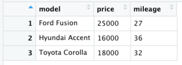
Figure 1.1: A view of the cars data frame generated by the View() function.
Each of the columns in the data frame contains one of the variables, with the name that we gave it when we created the data frame. We can access each of those columns using the $ operator. For example, if we wanted to access the mileage variable, we would combine the name of the data frame with the name of the variable as follows:
> cars_df$mileage
[1] 27 36 32
This is just like any other vector, in that we can refer to its individual values using square brackets as we did with regular vectors:
> cars_df$mileage[3]
[1] 32
In some of the examples in the book, you will see something called a tibble; this is basically a souped-up version of a data frame, and can be treated mostly in the same way.
1.9 Using R libraries
Many of the useful features in R are not contained in the primary R package, but instead come from libraries that have been developed by various members of the R community. For example, the ggplot2 package provides a number of features for visualizing data, as we will see in a later chapter. Before we can use a package, we need to install it on our system, using the install.packages() function:
> install.packages("ggplot2")
trying URL 'https://cran.rstudio.com/...
Content type 'application/x-gzip' length 3961383 bytes (3.8 MB)
==================================================
downloaded 3.8 MB


The downloaded binary packages are in
    /var/folders/.../downloaded_packages
This will automatically download the package from the Comprehensive R Archive Network (CRAN) and install it on your system. Once it’s installed, you can then load the library using the library() function:
> library(ggplot2)After loading the function, you can now access all of its features. If you want to learn more about its features, you can find them using the help function:
> help(ggplot2)1.10 Working with data files
When we are doing statistics, we often need to load in the data that we will analyze. Those data will live in a file on one’s computer or on the internet. For this example, let’s use a file that is hosted on the internet, which contains the gross domestic product (GDP) values for a number of countries around the world. This file is stored as comma-delimited text, meaning that the values for each of the variables in the dataset are separate by commas. There are three variables: the relative rank of the countries, the name of the country, and its GDP value. Here is what the first few lines of the file look like:
Rank,Country,GDP
1,Liechtenstein,141100
2,Qatar,104300
3,Luxembourg,81100
We can load a comma-delimited text file into R using the read.csv() function, which will accept either the location of a file on one’s computer, or a URL for files that are located on the web:
url < 'https://raw.githubusercontent.com/psych10/psych10/master/notebooks/Session03-IntroToR/gdp.csv'
gdp_df <- read.csv(url)
Once you have done this, take a look at the data frame using the View() function, and make sure that it looks right — it should have a column for each of the three variables.
Let’s say that we wanted to create a new file, which contained GDP values in Euros rather than US Dollars. We use today’s exchange rate, which is 1 USD == 0.90 Euros. To convert from Dollars to Euros, we simply multiple the GDP values by the exchange rate, and assign those values to a new variable within the data frame:
> exchange_rate <- 0.9
> gdp_df$GDP_euros <- gdp_df$GDP * exchange_rate
You should now see a new variable within the data frame, called “GDP_euros” which contains the new values. Now let’s save this to a comma-delimited text file on our computer called “gdp_euro.csv”.
We do this using the write.table() command.
> write.table(gdp_df, file='gdp_euro.csv')
This file will be created with the working directory that RStudio is using. You can find this directory using the getwd() function:
> getwd()
[1] "/Users/me/MyClasses/Psych10/LearningR"
1.11 Learning objectives
Having finished this chapter, you should be able to:
- Interact with an RMarkdown notebook in RStudio
- Describe the difference between a variable and a function
- Describe the different types of variables
- Create a vector or data frame and access its elements
- Install and load an R library
- Load data from a file and view the data frame
1.12 Suggested readings and videos
There are many online resources for learning R. Here are a few:
- Datacamp: Offers free online courses for many aspects of R programming
- A Student’s Guide to R
- R for cats: A humorous introduction to R programming
- aRrgh: a newcomer’s (angry) guide to R
- Quick-R
- RStudio Cheat Sheets: Quick references for many different aspects of R programming
- tidverse Style Guide: Make your code beautiful and reader-friendly!
- R for Data Science: This free online book focuses on working with data in R.
- Advanced R: This free online book by Hadley Wickham will help you get to the next level once your R skills start to develop.
- R intro for Python users: Used Python before? Check this out for a guide on how to transition to R.