Resampling and simulation

Generating random samples

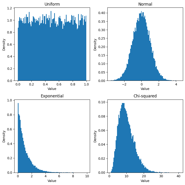
Here we will generate random samples from a number of different distributions and plot their histograms. We could write out separate commands to plot each of our functions of interest, but that would involve repeating a lot of code, so instead we will take advantage of the fact that Python allows us to treat modules as variables. We will specify the module that creates each distribution, and then loop through them, each time incrementing the panel number. Some distributions also take specific parameters; for example, the Chi-squared distribution requires specifying the degrees of freedom. We will store those in a separate dictionary and use them as needed.

import scipy.stats
import matplotlib.pyplot as plt

num_samples = 10000

plt.figure(figsize=(8, 8))

generators = {'Uniform': scipy.stats.uniform,
              'Normal': scipy.stats.norm, 
              'Exponential': scipy.stats.expon,
              'Chi-squared': scipy.stats.chi2}

generator_parameters = {'Chi-squared': 10}
panel_num = 1
for distribution in generators:
    plt.subplot(2, 2, panel_num)
    if distribution in generator_parameters:
        sample = generators[distribution].rvs(
            generator_parameters[distribution], size=num_samples)
    else:
        sample = generators[distribution].rvs(size=num_samples)
    plt.hist(sample, bins=100)
    plt.title(distribution)
    plt.xlabel('Value')
    plt.ylabel('Density')
    # the following function prevents the labels from overlapping
    plt.tight_layout()
    panel_num += 1

Simulating the maximum finishing time

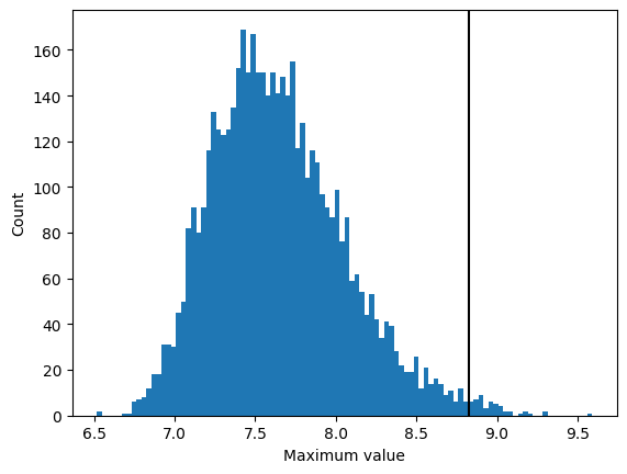
Let’s simulate 5000 samples of 150 observations, collecting the maximum value from each sample, and then plotting the distribution of maxima.

import numpy as np
import pandas as pd

num_runs = 5000
sample_size = 150


def sample_and_return_max(sample_size, 
                          distribution=None):
    """
    function to sample from a distribution and return maximum
    """

    # if distribution is not specified, then use the normal
    if distribution is None:
        distribution = scipy.stats.norm
    
    sample = distribution.rvs(size=sample_size)
    return(np.max(sample))


sample_max_df = pd.DataFrame({'max': np.zeros(num_runs)})

for i in range(num_runs):
    sample_max_df.loc[i, 'max'] = sample_and_return_max(sample_size)

Now let’s find the 95th percentile of the maximum distriibution. There is a built-in function in the scipy.stats module, called scoreatpercentile that will do this for us:

cutoff = scipy.stats.scoreatpercentile(sample_max_df['max'], 95)

Plot the histogram of the maximum values, along with a vertical line at the 95th percentile.

hist = plt.hist(sample_max_df['max'], bins=100)
plt.ylabel('Count')
plt.xlabel('Maximum value')
_ = plt.axvline(x=cutoff, ymax=np.max(hist[0]), color='k')

The bootstrap

The bootstrap is useful for creating confidence intervals in cases where we don’t have a parametric distribution. One example is for the median; let’s look at how that works. We will start by implementing it by hand, to see more closely how it works. We will start by collecting a sample of individuals from the NHANES dataset, and the using the bootstrap to obtain confidence intervals on the median for the Height variable.

#+
from nhanes.load import load_NHANES_data
nhanes_data = load_NHANES_data()
adult_nhanes_data = nhanes_data.query('AgeInYearsAtScreening > 17')
adult_nhanes_data = adult_nhanes_data.dropna(subset=['StandingHeightCm']).rename(columns={'StandingHeightCm': 'Height'})

num_runs = 5000
sample_size = 100

# Take a sample for which we will perform the bootstrap

nhanes_sample = adult_nhanes_data.sample(sample_size)

# Perform the resampling

bootstrap_df = pd.DataFrame({'mean': np.zeros(num_runs)})
for sampling_run in range(num_runs):
    bootstrap_sample = nhanes_sample.sample(sample_size, replace=True)
    bootstrap_df.loc[sampling_run, 'mean'] = bootstrap_sample['Height'].mean()

# Compute the 2.5% and 97.5% percentiles of the distribution


bootstrap_ci = [scipy.stats.scoreatpercentile(bootstrap_df['mean'], 2.5),
                scipy.stats.scoreatpercentile(bootstrap_df['mean'], 97.5)]

#-

Let’s compare the bootstrap distribution to the sampling distribution that we would expect given the sample mean and standard deviation:

# hist = plt.hist(bootstrap_df['mean'], 100, density=True)
#
# hist_bin_min = np.min(hist[1])
# hist_bin_max = np.max(hist[1])
# step_size = 0.01
# x_values = np.arange(hist_bin_min, hist_bin_max, step_size)
# normal_values = scipy.stats.norm.pdf(
#     x_values,
#     loc=nhanes_sample['Height'].mean(),
#     scale=nhanes_sample['Height'].std()/np.sqrt(sample_size))
# plt.plot(x_values, normal_values, color='r')
#
#

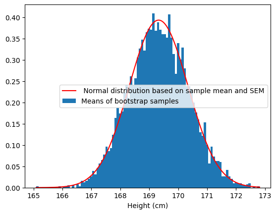
This shows that the bootstrap sampling distrbution does a good job of recapitulating the theoretical sampling distribution in this case.