The General Linear Model

The General Linear Model#

In this chapter we will explore how to fit general linear models in Python. We will focus on the tools provided by the statsmodels package.

from nhanes.load import load_NHANES_data
nhanes_data = load_NHANES_data()
adult_nhanes_data = nhanes_data.query('AgeInYearsAtScreening > 17')

Linear regression#

To perform linear regression in Python, we use the OLS() function (which stands for ordinary least squares) from the statsmodels package. Let’s generate some simulated data and use this function to compute the linear regression solution.

import numpy as np
import pandas as pd
import matplotlib.pyplot as plt


def generate_linear_data(slope, intercept,
                         noise_sd=1, x=None, 
                         npoints=100, seed=None):
    """
    generate data with a given slope and intercept
    and add normally distributed noise

    if x is passed as an argument then a given x will be used,
    otherwise it will be generated randomly

    Returns:
    --------
    a pandas data frame with variables x and y
    """
    if seed is not None:
        np.random.seed(seed)
    if x is None:
        x = np.random.randn(npoints)
    
    y = x * slope + intercept + np.random.randn(x.shape[0]) * noise_sd
    return(pd.DataFrame({'x': x, 'y': y}))


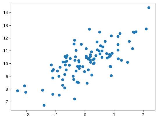
slope = 1
intercept = 10
noise_sd = 1
simulated_data = generate_linear_data(slope, intercept, noise_sd, seed=1)

plt.scatter(simulated_data['x'], simulated_data['y'])

<matplotlib.collections.PathCollection at 0x7f9e5cdc2d80>

_images/52b4a700144d39470dd1ef18cb796f381a9edfa8d0fac57763a542cb53d73248.png

We can then perform linear regression on these data using the ols function. This function doesn’t automatically include an intercept in its model, so we need to add one to the design. Fitting the model using this function is a two-step process. First, we set up the model and store it to a variable (which we will call ols_model). Then, we actually fit the model, which generates the results that we store to a different variable called ols_results, and view a summary using the .summary() method of the results variable.

from statsmodels.formula.api import ols

ols_model = ols(formula='y ~ x + 1', data=simulated_data)
ols_result = ols_model.fit()
ols_result.summary()

---------------------------------------------------------------------------
ModuleNotFoundError                       Traceback (most recent call last)
Cell In[3], line 1
----> 1 from statsmodels.formula.api import ols
      3 ols_model = ols(formula='y ~ x + 1', data=simulated_data)
      4 ols_result = ols_model.fit()

ModuleNotFoundError: No module named 'statsmodels'

We should see three things in these results:

The estimate of the Intercept in the model should be very close to the intercept that we specified
The estimate for the x parameter should be very close to the slope that we specified
The residual standard deviation should be roughly similar to the noise standard deviation that we specified. The summary doesn’t report the residual standard deviation directly but we can compute it using the residuals that are stored in the .resid element in the result output:

ols_result.resid.std()

Model criticism and diagnostics#

Once we have fitted the model, we want to look at some diagnostics to determine whether the model is actually fitting properly.
The first thing to examine is to make sure that the residuals are (at least roughly) normally distributed. We can do this using a Q-Q plot:

import seaborn as sns
import scipy.stats

_ = scipy.stats.probplot(ols_result.resid, plot=sns.mpl.pyplot)

This looks pretty good, in the sense that the residual data points fall very close to the unit line. This is not surprising, since we generated the data with normally distributed noise. We should also plot the predicted (or fitted) values against the residuals, to make sure that the model does work systematically better for some predicted values versus others.

plt.scatter(ols_result.fittedvalues, ols_result.resid)
plt.xlabel('Fitted value')
plt.ylabel('Residual')

As expected, we see no clear relationship.

Examples of problematic model fit#

Let’s say that there was another variable at play in this dataset, which we were not aware of. This variable causes some of the cases to have much larger values than others, in a way that is unrelated to the X variable. We play a trick here using the seq() function to create a sequence from zero to one, and then threshold those 0.5 (in order to obtain half of the values as zero and the other half as one) and then multiply by the desired effect size:

simulated_data.loc[:, 'x2'] = (simulated_data.index < (simulated_data.shape[0] / 2)).astype('int')
hidden_effect_size = 10
simulated_data.loc[:, 'y2'] = simulated_data['y'] + simulated_data['x2'] * hidden_effect_size

Now we fit the model again, and examine the residuals:

ols_model2 = ols(formula='y2 ~ x + 1', data=simulated_data)
ols_result2 = ols_model2.fit()

plt.figure(figsize=(12, 6))
plt.subplot(1, 2, 1)
scipy.stats.probplot(ols_result2.resid, plot=sns.mpl.pyplot)

plt.subplot(1, 2, 2)
plt.scatter(ols_result2.fittedvalues, ols_result2.resid)
plt.xlabel('Fitted value')
plt.ylabel('Residual')

The lack of normality is clear from the Q-Q plot, and we can also see that there is obvious structure in the residuals.

Let’s look at another potential problem, in which the y variable is nonlinearly related to the X variable. We can create these data by squaring the X variable when we generate the Y variable:

noise_sd = 0.1
simulated_data['y3'] = (simulated_data['x']**2) * slope + intercept + np.random.randn(simulated_data.shape[0]) * noise_sd

plt.scatter(simulated_data['x'], simulated_data['y3'])

ols_model3 = ols(formula='y3 ~ x + 1', data=simulated_data)
ols_result3 = ols_model3.fit()
ols_result3.summary()

Now we see that there is no significant linear relationship between \(X^2\) and Y/ But if we look at the residuals the problem with the model becomes clear:

plt.figure(figsize=(12, 6)) plt.subplot(1, 2, 1) scipy.stats.probplot(ols_result3.resid, plot=sns.mpl.pyplot)

plt.subplot(1, 2, 2) plt.scatter(ols_result3.fittedvalues, ols_result3.resid) plt.xlabel(‘Fitted value’) plt.ylabel(‘Residual’)

In this case we can see the clearly nonlinear relationship between the predicted and residual values, as well as the clear lack of normality in the residuals.

As we noted in the previous chapter, the “linear” in the general linear model doesn’t refer to the shape of the response, but instead refers to the fact that model is linear in its parameters — that is, the predictors in the model only get multiplied the parameters (e.g., rather than being raised to a power of the parameter). Here is how we would build a model that could account for the nonlinear relationship, by using x**2 in the model:

simulated_data.loc[:, 'x_squared'] = simulated_data['x'] ** 2
ols_model4 = ols(formula='y3 ~ x_squared + 1', data=simulated_data)
ols_result4 = ols_model4.fit()
ols_result4.summary()

Now we see that the effect of \(X^2\) is significant, and if we look at the residual plot we should see that things look much better:

plt.figure(figsize=(12, 6))
plt.subplot(1, 2, 1)
scipy.stats.probplot(ols_result4.resid, plot=sns.mpl.pyplot)

plt.subplot(1, 2, 2)
plt.scatter(ols_result4.fittedvalues, ols_result4.resid)
plt.xlabel('Fitted value')
plt.ylabel('Residual')

Not perfect, but much better than before!

Extending regression to binary outcomes.#

from statsmodels.formula.api import logit

diabetes_df = adult_nhanes_data.query(
    'DoctorToldYouHaveDiabetes != "Borderline"').dropna(
        subset=['DoctorToldYouHaveDiabetes', 'AgeInYearsAtScreening', 'BodyMassIndexKgm2']).rename(
            columns={'DoctorToldYouHaveDiabetes': 'Diabetes', 'AgeInYearsAtScreening': 'Age', 'BodyMassIndexKgm2': 'BMI'})
diabetes_df.loc[:, 'Diabetes'] = diabetes_df['Diabetes'].astype('int')

Now we would like to build a model that allows us to predict who has diabetes, based on their age and Body Mass Index (BMI). However, you may have noticed that the Diabetes variable is a binary variable; because linear regression assumes that the residuals from the model will be normally distributed, and the binary nature of the data will violate this, we instead need to use a different kind of model, known as a logistic regression model, which is built to deal with binary outcomes. We can fit this model using the logit() function:

logitfit = logit(formula = 'Diabetes ~ Age + BMI', data = diabetes_df).fit(disp=0)

logitfit.summary()

This looks very similar to the output from the ols() function, and it shows us that there is a significant relationship between the age, weight, and diabetes. The model provides us with a predicted probability that each individual will have diabetes; if this is greater than 0.5, then that means that the model predicts that the individual is more likely than not to have diabetes.
We can start by simply comparing those predictions to the actual outcomes.

diabetes_df.loc[:, 'LogitPrediction'] = (logitfit.predict() > 0.5).astype('int')

pd.crosstab(diabetes_df['Diabetes'], diabetes_df['LogitPrediction'])

This table shows that the model did somewhat well, in that it labeled most non-diabetic people as non-diabetic, and most diabetic people as diabetic. However, it also made a lot of mistakes, mislabeling nearly half of all diabetic people as non-diabetic.

We would often like a single number that tells us how good our prediction is. We could simply ask how many of our predictions are correct on average:

(diabetes_df['LogitPrediction'] == diabetes_df['Diabetes']).mean()

This tells us that we are doing fairly well at prediction, with over 80% accuracy. However, this measure is problematic, because most people in the sample don’t have diabetes. This means that we could get relatively high accuracy if we simply said that no one has diabetes:

(np.zeros(diabetes_df.shape[0]) == diabetes_df['Diabetes']).mean()

One commonly used value when we have a graded prediction (as we do here, with the probabiilty that is predicted by the model) is called the area under the receiver operating characteristic or AUROC. This is a number that ranges from zero to one, where 0.5 means that we are guessing, and one means that our predictions are perfect. Let’s see what that comes out to for this dataset, using the roc_auc_score from the scikit-learn package:

from sklearn.metrics import roc_auc_score
rocscore = roc_auc_score(diabetes_df['Diabetes'], logitfit.predict())
rocscore

Our model performs relatively well according to this score. What if we wanted to know whether this is better than chance? One option would be to create a null model, in which we purposely break the relationship between our variables. We could then ask how likely our observed score would be if there is no true relationship.

from sklearn.utils import shuffle

shuffled_df = diabetes_df.copy()

num_runs = 1000

roc_scores = pd.DataFrame({'auc': np.zeros(num_runs)})

for simulation_run in range(num_runs):
    # shuffle the diabetes labels in order to break the relationship
    shuffled_df.loc[:, 'Diabetes'] = shuffle(shuffled_df['Diabetes'].values)
    randomfit = logit(formula = 'Diabetes ~ Age + BMI', data = shuffled_df).fit(disp=0)
    roc_scores.loc[simulation_run, 'auc'] = roc_auc_score(shuffled_df['Diabetes'], randomfit.predict())

pvalue = (100 - scipy.stats.percentileofscore(roc_scores['auc'], rocscore))/100
pvalue

This shows us that our observed score is higher than all of 1000 scores obtained using random permutations. Thus, we can conclude that our accuracy is greater than chance. However, this doesn’t tell us how well we can predict whether a new individual will have diabetes. This is what we turn to next.

Cross-validation#

Cross-validation is a powerful technique that allows us to estimate how well our results will generalize to a new dataset. Here we will build our own crossvalidation code to see how it works, continuing the logistic regression example from the previous section. In cross-validation, we want to split the data into several subsets and then iteratively train the model while leaving out each subset (which we usually call folds) and then test the model on that held-out fold. We can use one of the tools from the scikit-learn package to create our cross-validation folds for us. Let’s start by using 10-fold crossvalidation, in which we split the data into 10 parts, and the fit the model while holding out one of those parts and then testing it on the held-out data.

from sklearn.model_selection import KFold

kf = KFold(n_splits=10, shuffle=True)

diabetes_df['Predicted'] = np.nan

for train_index, test_index in kf.split(diabetes_df):
    train_data = diabetes_df.iloc[train_index, :]
    test_data = diabetes_df.iloc[test_index, :]
    model = logit(formula = 'Diabetes ~ Age + BMI', data = train_data)
    trainfit = model.fit(disp=0)
    diabetes_df['Predicted'].iloc[list(test_index)] = trainfit.predict(
       test_data[['Age', 'BMI']])

print(pd.crosstab(diabetes_df['Diabetes'], diabetes_df['Predicted']>0.5))

roc_auc_score(diabetes_df['Diabetes'], diabetes_df['Predicted'])

This result shows that our model is able to generalize to new individuals relatively well — in fact, almost as well as the original model. This is because our sample size is very large; with smaller samples, the generalization performance is usually much less using crossvalidation than using the full sample.