Bayesian Statistics in Python

In this chapter we will introduce how to basic Bayesian computations using Python.

Applying Bayes’ theorem: A simple example

TBD: MOVE TO MULTIPLE TESTING EXAMPLE SO WE CAN USE BINOMIAL LIKELIHOOD A person has a cough and flu-like symptoms, and gets a PCR test for COVID-19, which comes back postiive. What is the likelihood that they actually have COVID-19, as opposed to a regular cold or flu? We can use Bayes’ theorem to compute this. Let’s say that the local rate of symptomatic individuals who actually are infected with COVID-19 is 7.4% (as reported on July 10, 2020 for San Francisco); thus, our prior probability that someone with symptoms actually has COVID-19 is .074. The RT-PCR test used to identify COVID-19 RNA is highly specific (that is, it very rarelly reports the presence of the virus when it is not present); for our example, we will say that the specificity is 99%. Its sensitivity is not known, but probably is no higher than 90%.
First let’s look at the probability of disease given a single positive test.

sensitivity = 0.90
specificity = 0.99
prior = 0.074
likelihood = sensitivity  # p(test|disease present) 
marginal_likelihood = sensitivity * prior + (1 - specificity) * (1 - prior)
posterior = (likelihood * prior) / marginal_likelihood
posterior

0.8779330345373055

The high specificity of the test, along with the relatively high base rate of the disease, means that most people who test positive actually have the disease. Now let’s plot the posterior as a function of the prior. Let’s first create a function to compute the posterior, and then apply this with a range of values for the prior.

import numpy as np
import pandas as pd
import scipy.stats
import matplotlib.pyplot as plt


def compute_posterior(prior, sensitivity, specificity):
    likelihood = sensitivity  # p(test|disease present) 
    marginal_likelihood = sensitivity * prior + (1 - specificity) * (1 - prior)
    posterior = (likelihood * prior) / marginal_likelihood
    return(posterior)


prior_values = np.arange(0.001, 0.5, 0.001)
posterior_values = compute_posterior(prior_values, sensitivity, specificity)

plt.plot(prior_values, posterior_values)
plt.xlabel('prior')
_ = plt.ylabel('posterior')

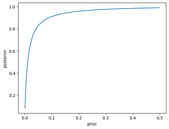
This figure highlights a very important general point about diagnostic testing: Even when the test has high specificity, if a condition is rare then most positive test results will be false positives.

Estimating posterior distributions

In this example we will look at how to estimate entire posterior distributions.
We will implement the drug testing example from the book. In that example, we administered a drug to 100 people, and found that 64 of them responded positively to the drug. What we want to estimate is the probability distribution for the proportion of responders, given the data. For simplicity we started with a uniform prior; that is, all proprtions of responding are equally likely to begin with. In addition, we will use a discrete probability distribution; that is, we will estimate the posterior probabiilty for each particular proportion of responders, in steps of 0.01. This greatly simplifies the math and still retains the main idea.

#+
num_responders = 64
num_tested = 100

bayes_df = pd.DataFrame({'proportion': np.arange(0.0, 1.01, 0.01)})

# compute the binomial likelihood of the observed data for each
# possible value of proportion
bayes_df['likelihood'] = scipy.stats.binom.pmf(num_responders,
                                               num_tested,
                                               bayes_df['proportion'])
# The prior is equal for all possible values
bayes_df['prior'] = 1 / bayes_df.shape[0]

# compute the marginal likelihood by adding up the likelihood of each possible proportion times its prior probability.

marginal_likelihood = (bayes_df['likelihood'] * bayes_df['prior']).sum()

bayes_df['posterior'] = (bayes_df['likelihood'] * bayes_df['prior']) / marginal_likelihood

# plot the likelihood, prior, and posterior

plt.plot(bayes_df['proportion'], bayes_df['likelihood'], label='likelihood')
plt.plot(bayes_df['proportion'], bayes_df['prior'], label='prior')
plt.plot(bayes_df['proportion'], bayes_df['posterior'],
         'k--', label='posterior')

plt.legend()

#-

<matplotlib.legend.Legend at 0x7fd44344b050>

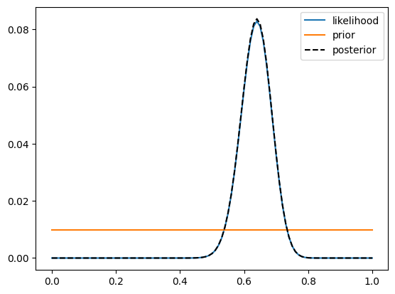
The plot shows that the posterior and likelihood are virtually identical, which is due to the fact that the prior is uniform across all possible values. Now let’s look at a case where the prior is not uniform. Let’s say that we now run a larger study of 1000 people with the same treatment, and we find that 312 of the 1000 individuals respond to the treatment. In this case, we can use the posterior from the earlier study of 100 people as the prior for our new study. This is what we sometimes refer to as Bayesian updating.

#+
num_responders = 312
num_tested = 1000

# copy the posterior from the previous analysis and rename it as the prior

study2_df = bayes_df[['proportion', 'posterior']].rename(columns={'posterior': 'prior'})

# compute the binomial likelihood of the observed data for each
# possible value of proportion

study2_df['likelihood'] = scipy.stats.binom.pmf(num_responders,
                                               num_tested,
                                               study2_df['proportion'])

# compute the marginal likelihood by adding up the likelihood of each possible proportion times its prior probability.

marginal_likelihood = (study2_df['likelihood'] * study2_df['prior']).sum()

study2_df['posterior'] = (study2_df['likelihood'] * study2_df['prior']) / marginal_likelihood

# plot the likelihood, prior, and posterior

plt.plot(study2_df['proportion'], study2_df['likelihood'], label='likelihood')
plt.plot(study2_df['proportion'], study2_df['prior'], label='prior')
plt.plot(study2_df['proportion'], study2_df['posterior'],
         'k--', label='posterior')

plt.legend()

#-

<matplotlib.legend.Legend at 0x7fd44344b2c0>

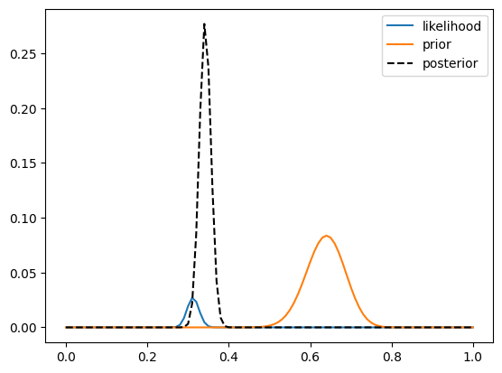
Here we see two important things. First, we see that the prior is substantially wider than the likelihood, which occurs because there is much more data going into the likelihood (1000 data points) compared to the prior (100 data points), and more data reduces our uncertainty. Second, we see that the posterior is much closer to the value observed for the second study than for the first, which occurs for the same reason — we put greater weight on the estimate that is more precise due to a larger sample.

Bayes factors

There are no convenient off-the-shelf tools for estimating Bayes factors using Python, so we will use the rpy2 package to access the BayesFactor library in R. Let’s compute a Bayes factor for a T-test comparing the amount of reported alcohol computing between smokers versus non-smokers. First, let’s set up the NHANES data and collect a sample of 150 smokers and 150 nonsmokers.

#+
from nhanes.load import load_NHANES_data
nhanes_data = load_NHANES_data()
adult_nhanes_data = nhanes_data.query('AgeInYearsAtScreening > 17')
rseed = 1

# clean up smoking variables
adult_nhanes_data.loc[adult_nhanes_data['SmokedAtLeast100CigarettesInLife'] == 0, 'DoYouNowSmokeCigarettes'] = 'Not at all'
adult_nhanes_data.loc[:, 'SmokeNow'] = adult_nhanes_data['DoYouNowSmokeCigarettes'] != 'Not at all'

# Create average alcohol consumption variable between the two dietary recalls
adult_nhanes_data.loc[:, 'AvgAlcohol'] = adult_nhanes_data[['AlcoholGm_DR1TOT', 'AlcoholGm_DR2TOT']].mean(1)
adult_nhanes_data = adult_nhanes_data.dropna(subset=['AvgAlcohol'])

sample_size_per_group = 150

nonsmoker_sample = adult_nhanes_data.query('SmokeNow == False').sample(sample_size_per_group, random_state=rseed)[['SmokeNow', 'AvgAlcohol']]
smoker_sample = adult_nhanes_data.query('SmokeNow == True').sample(sample_size_per_group, random_state=rseed)[['SmokeNow', 'AvgAlcohol']]

full_sample = pd.concat((nonsmoker_sample, smoker_sample))
full_sample.loc[:, 'SmokeNow'] = full_sample['SmokeNow'].astype('int')
full_sample.groupby('SmokeNow').mean()
#-

/tmp/ipykernel_351/61854950.py:9: SettingWithCopyWarning: 
A value is trying to be set on a copy of a slice from a DataFrame.
Try using .loc[row_indexer,col_indexer] = value instead

See the caveats in the documentation: https://pandas.pydata.org/pandas-docs/stable/user_guide/indexing.html#returning-a-view-versus-a-copy
  adult_nhanes_data.loc[:, 'SmokeNow'] = adult_nhanes_data['DoYouNowSmokeCigarettes'] != 'Not at all'
/tmp/ipykernel_351/61854950.py:12: SettingWithCopyWarning: 
A value is trying to be set on a copy of a slice from a DataFrame.
Try using .loc[row_indexer,col_indexer] = value instead

See the caveats in the documentation: https://pandas.pydata.org/pandas-docs/stable/user_guide/indexing.html#returning-a-view-versus-a-copy
  adult_nhanes_data.loc[:, 'AvgAlcohol'] = adult_nhanes_data[['AlcoholGm_DR1TOT', 'AlcoholGm_DR2TOT']].mean(1)

	AvgAlcohol
SmokeNow
0	5.748000
1	11.875333

Now let’s use functions from R to perform a standard t-test as well as compute a Bayes Factor for this comparison.

#+

# import the necessary functions from rpy2
import rpy2.robjects as robjects
from rpy2.robjects import r, pandas2ri
from rpy2.robjects.packages import importr
pandas2ri.activate()

# import the BayesFactor package
BayesFactor = importr('BayesFactor')

# import the data frames into the R workspace
robjects.globalenv["smoker_sample"] = smoker_sample
robjects.globalenv["nonsmoker_sample"] = nonsmoker_sample

# perform the standard t-test
ttest_output = r('print(t.test(smoker_sample$AvgAlcohol, nonsmoker_sample$AvgAlcohol, alternative="greater"))')

# compute the Bayes factor
r('bf = ttestBF(y=nonsmoker_sample$AvgAlcohol, x=smoker_sample$AvgAlcohol, nullInterval = c(0, Inf))')
r('print(bf[1]/bf[2])')

#-

---------------------------------------------------------------------------
ModuleNotFoundError                       Traceback (most recent call last)
Cell In[6], line 4
      1 #+
      2 
      3 # import the necessary functions from rpy2
----> 4 import rpy2.robjects as robjects
      5 from rpy2.robjects import r, pandas2ri
      6 from rpy2.robjects.packages import importr

ModuleNotFoundError: No module named 'rpy2'

This shows that the difference between these groups is significant, and the Bayes factor suggests fairly strong evidence for a difference.