Chapter 11 Bayesian statistics

In this chapter we will take up the approach to statistical modeling and inference that stands in contrast to the null hypothesis testing framework that you encountered in Chapter 9. This is known as “Bayesian statistics” after the Reverend Thomas Bayes, whose theorem you have already encountered in Chapter 6. In this chapter you will learn how Bayes’ theorem provides a way of understanding data that solves many of the conceptual problems that we discussed regarding null hypothesis testing, while also introducing some new challenges.

11.1 Generative models

Say you are walking down the street and a friend of yours walks right by but doesn’t say hello. You would probably try to decide why this happened – Did they not see you? Are they mad at you? Are you suddenly cloaked in a magic invisibility shield? One of the basic ideas behind Bayesian statistics is that we want to infer the details of how the data are being generated, based on the data themselves. In this case, you want to use the data (i.e. the fact that your friend did not say hello) to infer the process that generated the data (e.g. whether or not they actually saw you, how they feel about you, etc).

The idea behind a generative model is that a latent (unseen) process generates the data we observe, usually with some amount of randomness in the process. When we take a sample of data from a population and estimate a parameter from the sample, what we are doing in essence is trying to learn the value of a latent variable (the population mean) that gives rise through sampling to the observed data (the sample mean). Figure 11.1 shows a schematic of this idea.

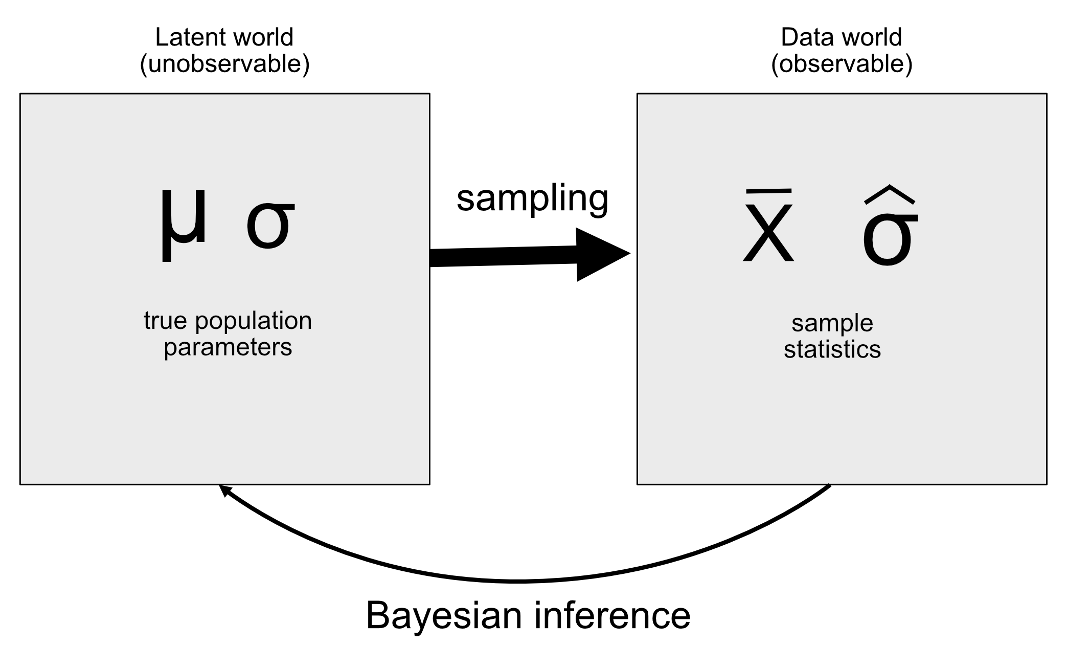
Figure 11.1: A schematic of the idea of a generative model.

If we know the value of the latent variable, then it’s easy to reconstruct what the observed data should look like. For example, let’s say that we are flipping a coin that we know to be fair, such that we would expect it to land on heads 50% of the time. We can describe the coin by a binomial distribution with a value of \(P_{heads}=0.5\), and then we could generate random samples from such a distribution in order to see what the observed data should look like. However, in general we are in the opposite situation: We don’t know the value of the latent variable of interest, but we have some data that we would like to use to estimate it.

11.2 Bayes’ theorem and inverse inference

The reason that Bayesian statistics has its name is because it takes advantage of Bayes’ theorem to make inferences from data about the underlying process that generated the data. Let’s say that we want to know whether a coin is fair. To test this, we flip the coin 10 times and come up with 7 heads. Before this test we were pretty sure that the \(P_{heads}=0.5\), but finding 7 heads out of 10 flips would certainly give us pause if we believed that \(P_{heads}=0.5\). We already know how to compute the conditional probability that we would flip 7 or more heads out of 10 if the coin is really fair (\(P(n\ge7|p_{heads}=0.5)\)), using the binomial distribution.

The resulting probability is 0.055. That is a fairly small number, but this number doesn’t really answer the question that we are asking – it is telling us about the likelihood of 7 or more heads given some particular probability of heads, whereas what we really want to know is the true probability of heads for this particular coin. This should sound familiar, as it’s exactly the situation that we were in with null hypothesis testing, which told us about the likelihood of data rather than the likelihood of hypotheses.

Remember that Bayes’ theorem provides us with the tool that we need to invert a conditional probability:

\[ P(H|D) = \frac{P(D|H)*P(H)}{P(D)} \]

We can think of this theorem as having four parts:

• prior (\(P(Hypothesis)\)): Our degree of belief about hypothesis H before seeing the data D
• likelihood (\(P(Data|Hypothesis)\)): How likely are the observed data D under hypothesis H?
• marginal likelihood (\(P(Data)\)): How likely are the observed data, combining over all possible hypotheses?
• posterior (\(P(Hypothesis|Data)\)): Our updated belief about hypothesis H, given the data D

In the case of our coin-flipping example:

• prior (\(P_{heads}\)): Our degree of belief about the likelhood of flipping heads, which was \(P_{heads}=0.5\)
• likelihood (\(P(\text{7 or more heads out of 10 flips}|P_{heads}=0.5)\)): How likely are 7 or more heads out of 10 flips if \(P_{heads}=0.5)\)?
• marginal likelihood (\(P(\text{7 or more heads out of 10 flips})\)): How likely are we to observe 7 heads out of 10 coin flips, in general?
• posterior (\(P_{heads}|\text{7 or more heads out of 10 coin flips})\)): Our updated belief about \(P_{heads}\) given the observed coin flips

Here we see one of the primary differences between frequentist and Bayesian statistics. Frequentists do not believe in the idea of a probability of a hypothesis (i.e. our degree of belief about a hypothesis) – for them, a hypothesis is either true or it isn’t. Another way to say this is that for the frequentist, the hypothesis is fixed and the data are random, which is why frequentist inference focuses on describing the probability of data given a hypothesis (i.e. the p-value). Bayesians, on the other hand, are comfortable making probability statements about both data and hypotheses.

11.3 Doing Bayesian estimation

We ultimately want to use Bayesian statistics to make decisions about hypotheses, but before we do that we need to estimate the parameters that are necessary to make the decision. Here we will walk through the process of Bayesian estimation. Let’s use another screening example: Airport security screening. If you fly a lot, it’s just a matter of time until one of the random explosive screenings comes back positive; I had the particularly unfortunate experience of this happening soon after September 11, 2001, when airport security staff were especially on edge.

What the security staff want to know is what is the likelihood that a person is carrying an explosive, given that the machine has given a positive test. Let’s walk through how to calculate this value using Bayesian analysis.

11.3.1 Specifying the prior

To use Bayes’ theorem, we first need to specify the prior probability for the hypothesis. In this case, we don’t know the real number but we can assume that it’s quite small. According to the FAA, there were 971,595,898 air passengers in the U.S. in 2017. Let’s say that one of those travelers was carrying an explosive in their bag — that would give a prior probability of 1 out of 971 million, which is very small! The security personnel may have reasonably held a stronger prior in the months after the 9/11 attack, so let’s say that their subjective belief was that one out of every million flyers was carrying an explosive.

11.3.2 Collect some data

The data are composed of the results of the explosive screening test. Let’s say that the security staff runs the bag through their testing apparatus 3 times, and it gives a positive reading on 3 of the 3 tests.

11.3.3 Computing the likelihood

We want to compute the likelihood of the data under the hypothesis that there is an explosive in the bag. Let’s say that we know (from the machine’s manufacturer) that the sensitivity of the test is 0.99 – that is, when a device is present, it will detect it 99% of the time. To determine the likelihood of our data under the hypothesis that a device is present, we can treat each test as a Bernoulli trial (that is, a trial with an outcome of true or false) with a probability of success of 0.99, which we can model using a binomial distribution.

11.3.4 Computing the marginal likelihood

We also need to know the overall likelihood of the data – that is, finding 3 positives out of 3 tests. Computing the marginal likelihood is often one of the most difficult aspects of Bayesian analysis, but for our example it’s simple because we can take advantage of the specific form of Bayes’ theorem for a binary outcome that we introduced in Section 6.7:

\[ P(E|T) = \frac{P(T|E)*P(E)}{P(T|E)*P(E) + P(T|\neg E)*P(\neg E)} \]

where \(E\) refers to the presence of explosives, and \(T\) refers to a postive test result.

The marginal likelihood in this case is a weighted average of the likelihood of the data under either presence or absence of the explosive, multiplied by the probability of the explosive being present (i.e. the prior). In this case, let’s say that we know (from the manufacturer) that the specificity of the test is 0.99, such that the likelihood of a positive result when there is no explosive (\(P(T|\neg E)\)) is 0.01.

11.3.5 Computing the posterior

We now have all of the parts that we need to compute the posterior probability of an explosive being present, given the observed 3 positive outcomes out of 3 tests.
This result shows us that the posterior probability of an explosive in the bag given these positive tests (0.492) is just under 50%, again highlighting the fact that testing for rare events is almost always liable to produce high numbers of false positives, even when the specificity and sensitivity are very high.

An important aspect of Bayesian analysis is that it can be sequential. Once we have the posterior from one analysis, it can become the prior for the next analysis!

11.4 Estimating posterior distributions

In the previous example there were only two possible outcomes – the explosive is either there or it’s not – and we wanted to know which outcome was most likely given the data. However, in other cases we want to use Bayesian estimation to estimate the numeric value of a parameter. Let’s say that we want to know about the effectiveness of a new drug for pain; to test this, we can administer the drug to a group of patients and then ask them whether their pain was improved or not after taking the drug. We can use Bayesian analysis to estimate the proportion of people for whom the drug will be effective using these data.

11.4.1 Specifying the prior

In this case, we don’t have any prior information about the effectiveness of the drug, so we will use a uniform distribution as our prior, since all values are equally likely under a uniform distribution. In order to simplify the example, we will only look at a subset of 99 possible values of effectiveness (from .01 to .99, in steps of .01). Therefore, each possible value has a prior probability of 1/99.

11.4.2 Collect some data

We need some data in order to estimate the effect of the drug. Let’s say that we administer the drug to 100 individuals, we find that 64 respond positively to the drug.

11.4.3 Computing the likelihood

We can compute the likelihood of the observed data under any particular value of the effectiveness parameter using the binomial density function. In Figure 11.2 you can see the likelihood curves over numbers of responders for several different values of \(P_{respond}\). Looking at this, it seems that our observed data are relatively more likely under the hypothesis of \(P_{respond}=0.7\), somewhat less likely under the hypothesis of \(P_{respond}=0.5\), and quite unlikely under the hypothesis of \(P_{respond}=0.3\). One of the fundamental ideas of Bayesian inference is that we should upweight our belief in values of our parameter of interest in proportion to how likely the data are under those values, balanced against what we believed about the parameter values before having seen the data (our prior knowledge).

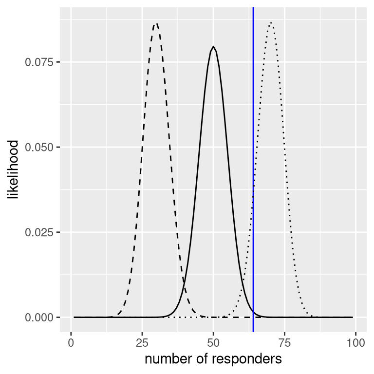
Figure 11.2: Likelihood of each possible number of responders under several different hypotheses (p(respond)=0.5 (solid), 0.7 (dotted), 0.3 (dashed). Observed value shown in the vertical line

11.4.4 Computing the marginal likelihood

In addition to the likelihood of the data under different hypotheses, we need to know the overall likelihood of the data, combining across all hypotheses (i.e., the marginal likelihood). This marginal likelihood is primarily important because it helps to ensure that the posterior values are true probabilities. In this case, our use of a set of discrete possible parameter values makes it easy to compute the marginal likelihood, because we can just compute the likelihood of each parameter value under each hypothesis and add them up.

11.4.5 Computing the posterior

We now have all of the parts that we need to compute the posterior probability distribution across all possible values of \(p_{respond}\), as shown in Figure 11.3.

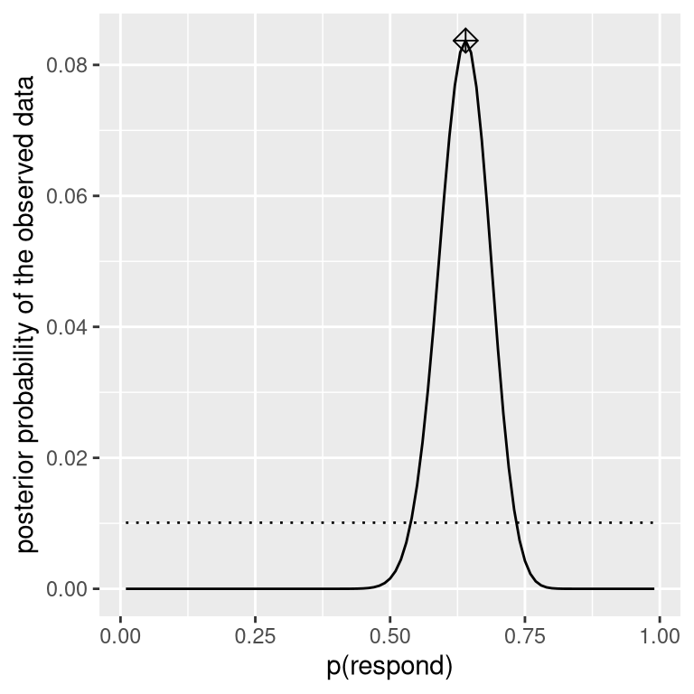
Figure 11.3: Posterior probability distribution for the observed data plotted in solid line against uniform prior distribution (dotted line). The maximum a posteriori (MAP) value is signified by the diamond symbol.

11.4.6 Maximum a posteriori (MAP) estimation

Given our data we would like to obtain an estimate of \(p_{respond}\) for our sample. One way to do this is to find the value of \(p_{respond}\) for which the posterior probability is the highest, which we refer to as the maximum a posteriori (MAP) estimate. We can find this from the data in 11.3 — it’s the value shown with a marker at the top of the distribution. Note that the result (0.64) is simply the proportion of responders from our sample – this occurs because the prior was uniform and thus didn’t influence our estimate.

11.4.7 Credible intervals

Often we would like to know not just a single estimate for the posterior, but an interval in which we are confident that the posterior falls. We previously discussed the concept of confidence intervals in the context of frequentist inference, and you may remember that the interpretation of confidence intervals was particularly convoluted: It was an interval that will contain the the value of the parameter 95% of the time. What we really want is an interval in which we are confident that the true parameter falls, and Bayesian statistics can give us such an interval, which we call a credible interval.

The interpretation of this credible interval is much closer to what we had hoped we could get from a confidence interval (but could not): It tells us that there is a 95% probability that the value of \(p_{respond}\) falls between these two values. Importantly, in this case it shows that we have high confidence that \(p_{respond} > 0.0\), meaning that the drug seems to have a positive effect.

In some cases the credible interval can be computed numerically based on a known distribution, but it’s more common to generate a credible interval by sampling from the posterior distribution and then to compute quantiles of the samples. This is particularly useful when we don’t have an easy way to express the posterior distribution numerically, which is often the case in real Bayesian data analysis. One such method (rejection sampling) is explained in more detail in the Appendix at the end of this chapter.

11.4.8 Effects of different priors

In the previous example we used a flat prior, meaning that we didn’t have any reason to believe that any particular value of \(p_{respond}\) was more or less likely. However, let’s say that we had instead started with some previous data: In a previous study, researchers had tested 20 people and found that 10 of them had responded positively. This would have lead us to start with a prior belief that the treatment has an effect in 50% of people. We can do the same computation as above, but using the information from our previous study to inform our prior (see panel A in Figure 11.4).

Note that the likelihood and marginal likelihood did not change - only the prior changed. The effect of the change in prior to was to pull the posterior closer to the mass of the new prior, which is centered at 0.5.

Now let’s see what happens if we come to the analysis with an even stronger prior belief. Let’s say that instead of having previously observed 10 responders out of 20 people, the prior study had instead tested 500 people and found 250 responders. This should in principle give us a much stronger prior, and as we see in panel B of Figure 11.4 , that’s what happens: The prior is much more concentrated around 0.5, and the posterior is also much closer to the prior. The general idea is that Bayesian inference combines the information from the prior and the likelihood, weighting the relative strength of each.

This example also highlights the sequential nature of Bayesian analysis – the posterior from one analysis can become the prior for the next analysis.

Finally, it is important to realize that if the priors are strong enough, they can completely overwhelm the data. Let’s say that you have an absolute prior that \(p_{respond}\) is 0.8 or greater, such that you set the prior likelihood of all other values to zero. What happens if we then compute the posterior?

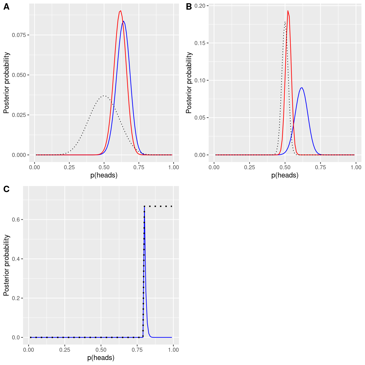
Figure 11.4: A: Effects of priors on the posterior distribution. The original posterior distribution based on a flat prior is plotted in blue. The prior based on the observation of 10 responders out of 20 people is plotted in the dotted black line, and the posterior using this prior is plotted in red. B: Effects of the strength of the prior on the posterior distribution. The blue line shows the posterior obtained using the prior based on 50 heads out of 100 people. The dotted black line shows the prior based on 250 heads out of 500 flips, and the red line shows the posterior based on that prior. C: Effects of the strength of the prior on the posterior distribution. The blue line shows the posterior obtained using an absolute prior which states that p(respond) is 0.8 or greater. The prior is shown in the dotted black line.

In panel C of Figure 11.4 we see that there is zero density in the posterior for any of the values where the prior was set to zero - the data are overwhelmed by the absolute prior.

11.5 Choosing a prior

The impact of priors on the resulting inferences are the most controversial aspect of Bayesian statistics. What is the right prior to use? If the choice of prior determines the results (i.e., the posterior), how can you be sure you results are trustworthy? These are difficult questions, but we should not back away just because we are faced with hard questions. As we discussed previously, Bayesian analyses give us interpretable results (credible intervals, etc.). This alone should inspire us to think hard about these questions so that we can arrive with results that are reasonable and interpretable.

There are various ways to choose one’s priors, which (as we saw above) can impact the resulting inferences. Sometimes we have a very specific prior, as in the case where we expected our coin to lands heads 50% of the time, but in many cases we don’t have such strong a starting point. Uninformative priors attempt to influence the resulting posterior as little as possible, as we saw in the example of the uniform prior above. It’s also common to use weakly informative priors (or default priors), which influence the result only very slightly. For example, if we had used a binomial distribution based on one heads out of two coin flips, the prior would have been centered around 0.5 but fairly flat, influencing the posterior only slightly. It is also possible to use priors based on the scientific literature or pre-existing data, which we would call empirical priors. In general, however, we will stick to the use of uninformative/weakly informative priors, since they raise the least concern about influencing our results.

11.6 Bayesian hypothesis testing

Having learned how to perform Bayesian estimation, we now turn to the use of Bayesian methods for hypothesis testing. Let’s say that there are two politicians who differ in their beliefs about whether the public is in favor an extra tax to support the national parks. Senator Smith thinks that only 40% of people are in favor of the tax, whereas Senator Jones thinks that 60% of people are in favor. They arrange to have a poll done to test this, which asks 1000 randomly selected people whether they support such a tax. The results are that 490 of the people in the polled sample were in favor of the tax. Based on these data, we would like to know: Do the data support the claims of one senator over the other,and by how much? We can test this using a concept known as the Bayes factor, which quantifies which hypothesis is better by comparing how well each predicts the observed data.

11.6.1 Bayes factors

The Bayes factor characterizes the relative likelihood of the data under two different hypotheses. It is defined as:

\[ BF = \frac{p(data|H_1)}{p(data|H_2)} \]

for two hypotheses \(H_1\) and \(H_2\). In the case of our two senators, we know how to compute the likelihood of the data under each hypothesis using the binomial distribution; let’s assume for the moment that our prior probability for each senator being correct is the same (\(P_{H_1} = P_{H_2} = 0.5\)). We will put Senator Smith in the numerator and Senator Jones in the denominator, so that a value greater than one will reflect greater evidence for Senator Smith, and a value less than one will reflect greater evidence for Senator Jones. The resulting Bayes Factor (3325.26) provides a measure of the evidence that the data provides regarding the two hypotheses - in this case, it tells us the data support Senator Smith more than 3000 times more strongly than they support Senator Jones.

11.6.2 Bayes factors for statistical hypotheses

In the previous example we had specific predictions from each senator, whose likelihood we could quantify using the binomial distribution. In addition, our prior probability for the two hypotheses was equal. However, in real data analysis we generally must deal with uncertainty about our parameters, which complicates the Bayes factor, because we need to compute the marginal likelihood (that is, an integrated average of the likelihoods over all possible model parameters, weighted by their prior probabilities). However, in exchange we gain the ability to quantify the relative amount of evidence in favor of the null versus alternative hypotheses.

Let’s say that we are a medical researcher performing a clinical trial for the treatment of diabetes, and we wish to know whether a particular drug reduces blood glucose compared to placebo. We recruit a set of volunteers and randomly assign them to either drug or placebo group, and we measure the change in hemoglobin A1C (a marker for blood glucose levels) in each group over the period in which the drug or placebo was administered. What we want to know is: Is there a difference between the drug and placebo?

First, let’s generate some data and analyze them using null hypothesis testing (see Figure 11.5). Then let’s perform an independent-samples t-test, which shows that there is a significant difference between the groups:

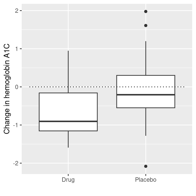
Figure 11.5: Box plots showing data for drug and placebo groups.

## 
##  Welch Two Sample t-test
## 
## data:  hbchange by group
## t = 2, df = 32, p-value = 0.02
## alternative hypothesis: true difference in means between group 0 and group 1 is greater than 0
## 95 percent confidence interval:
##  0.11  Inf
## sample estimates:
## mean in group 0 mean in group 1 
##          -0.082          -0.650

This test tells us that there is a significant difference between the groups, but it doesn’t quantify how strongly the evidence supports the null versus alternative hypotheses. To measure that, we can compute a Bayes factor using ttestBF function from the BayesFactor package in R:

## Bayes factor analysis
## --------------
## [1] Alt., r=0.707 0<d<Inf    : 3.4  ±0%
## [2] Alt., r=0.707 !(0<d<Inf) : 0.12 ±0.01%
## 
## Against denominator:
##   Null, mu1-mu2 = 0 
## ---
## Bayes factor type: BFindepSample, JZS

We are particularly interested in the Bayes Factor for an effect greater than zero, which is listed in the line marked “[1]” in the report. The Bayes factor here tells us that the alternative hypothesis (i.e. that the difference is greater than zero) is about 3 times more likely than the point null hypothesis (i.e. a mean difference of exactly zero) given the data. Thus, while the effect is significant, the amount of evidence it provides us in favor of the alternative hypothesis is rather weak.

11.6.2.1 One-sided tests

We generally are less interested in testing against the null hypothesis of a specific point value (e.g. mean difference = 0) than we are in testing against a directional null hypothesis (e.g. that the difference is less than or equal to zero). We can also perform a directional (or one-sided) test using the results from ttestBF analysis, since it provides two Bayes factors: one for the alternative hypothesis that the mean difference is greater than zero, and one for the alternative hypothesis that the mean difference is less than zero. If we want to assess the relative evidence for a positive effect, we can compute a Bayes factor comparing the relative evidence for a positive versus a negative effect by simply dividing the two Bayes factors returned by the function:

## Bayes factor analysis
## --------------
## [1] Alt., r=0.707 0<d<Inf : 29 ±0.01%
## 
## Against denominator:
##   Alternative, r = 0.707106781186548, mu =/= 0 !(0<d<Inf) 
## ---
## Bayes factor type: BFindepSample, JZS

Now we see that the Bayes factor for a positive effect versus a negative effect is substantially larger (almost 30).

11.6.2.2 Interpreting Bayes Factors

How do we know whether a Bayes factor of 2 or 20 is good or bad? There is a general guideline for interpretation of Bayes factors suggested by Kass & Rafferty (1995):

BF	Strength of evidence
1 to 3	not worth more than a bare mention
3 to 20	positive
20 to 150	strong
>150	very strong

Based on this, even though the statisical result is significant, the amount of evidence in favor of the alternative vs. the point null hypothesis is weak enough that it’s hardly worth even mentioning, whereas the evidence for the directional hypothesis is relatively strong.

11.6.3 Assessing evidence for the null hypothesis

Because the Bayes factor is comparing evidence for two hypotheses, it also allows us to assess whether there is evidence in favor of the null hypothesis, which we couldn’t do with standard null hypothesis testing (because it starts with the assumption that the null is true). This can be very useful for determining whether a non-significant result really provides strong evidence that there is no effect, or instead just reflects weak evidence overall.

11.7 Learning objectives

After reading this chapter, should be able to:

• Describe the main differences between Bayesian analysis and null hypothesis testing
• Describe and perform the steps in a Bayesian analysis
• Describe the effects of different priors, and the considerations that go into choosing a prior
• Describe the difference in interpretation between a confidence interval and a Bayesian credible interval

11.8 Suggested readings

• The Theory That Would Not Die: How Bayes’ Rule Cracked the Enigma Code, Hunted Down Russian Submarines, and Emerged Triumphant from Two Centuries of Controversy, by Sharon Bertsch McGrayne
• Doing Bayesian Data Analysis: A Tutorial Introduction with R, by John K. Kruschke

11.9 Appendix:

11.9.1 Rejection sampling

We will generate samples from our posterior distribution using a simple algorithm known as rejection sampling. The idea is that we choose a random value of x (in this case \(p_{respond}\)) and a random value of y (in this case, the posterior probability of \(p_{respond}\)) each from a uniform distribution. We then only accept the sample if \(y < f(x)\) - in this case, if the randomly selected value of y is less than the actual posterior probability of y. Figure 11.6 shows an example of a histogram of samples using rejection sampling, along with the 95% credible intervals obtained using this method (with the values presented in Table ??).

	x
2.5%	0.54
97.5%	0.73

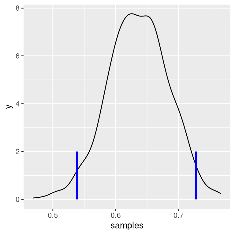
Figure 11.6: Rejection sampling example.The black line shows the density of all possible values of p(respond); the blue lines show the 2.5th and 97.5th percentiles of the distribution, which represent the 95 percent credible interval for the estimate of p(respond).