Chapter 17 Practical statistical modeling
In this chapter we will bring together everything that we have learned, by applying our knowledge to a practical example. In 2007, Christopher Gardner and colleagues from Stanford published a study in the Journal of the American Medical Association titled “Comparison of the Atkins, Zone, Ornish, and LEARN Diets for Change in Weight and Related Risk Factors Among Overweight Premenopausal Women – The A TO Z Weight Loss Study: A Randomized Trial” (Gardner et al. 2007). We will use this study to show how one would go about analyzing an experimental dataset from start to finish.
17.1 The process of statistical modeling
There is a set of steps that we generally go through when we want to use our statistical model to test a scientific hypothesis:
- Specify your question of interest
- Identify or collect the appropriate data
- Prepare the data for analysis
- Determine the appropriate model
- Fit the model to the data
- Criticize the model to make sure it fits properly
- Test hypothesis and quantify effect size
17.1.1 1: Specify your question of interest
According to the authors, the goal of their study was:
To compare 4 weight-loss diets representing a spectrum of low to high carbohydrate intake for effects on weight loss and related metabolic variables.
17.1.2 2: Identify or collect the appropriate data
To answer their question, the investigators randomly assigned each of 311 overweight/obese women to one of four different diets (Atkins, Zone, Ornish, or LEARN), and measured their weight along with many other measures of health over time. The authors recorded a large number of variables, but for the main question of interest let’s focus on a single variable: Body Mass Index (BMI). Further, since our goal is to measure lasting changes in BMI, we will only look at the measurement taken at 12 months after onset of the diet.
17.1.3 3: Prepare the data for analysis
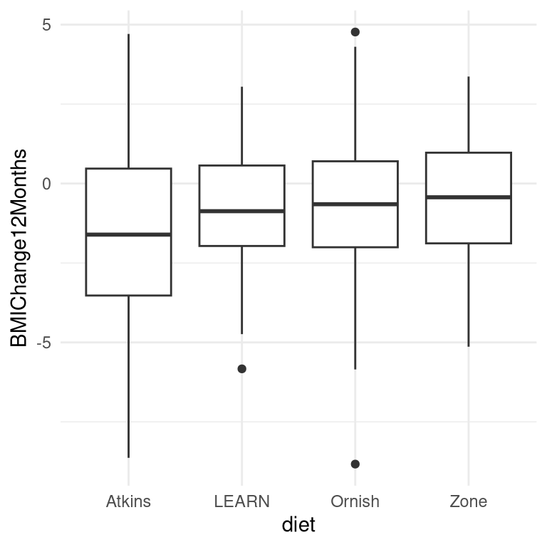
Figure 17.1: Box plots for each condition, with the 50th percentile (i.e the median) shown as a black line for each group.
The actual data from the A to Z study are not publicly available, so we will use the summary data reported in their paper to generate some synthetic data that roughly match the data obtained in their study, with the same means and standard deviations for each group. Once we have the data, we can visualize them to make sure that there are no outliers. Box plots are useful to see the shape of the distributions, as shown in Figure 17.1. Those data look fairly reasonable - there are a couple of outliers within individual groups (denoted by the dots outside of the box plots), but they don’t seem to be extreme with regard to the other groups. We can also see that the distributions seem to differ a bit in their variance, with Atkins showing somewhat greater variability than the others. This means that any analyses that assume the variances are equal across groups might be inappropriate. Fortunately, the ANOVA model that we plan to use is fairly robust to this.
17.1.4 4. Determine the appropriate model
There are several questions that we need to ask in order to determine the appropriate statistical model for our analysis.
- What kind of dependent variable?
- BMI: continuous, roughly normally distributed
- What are we comparing?
- mean BMI across four diet groups
- ANOVA is appropriate
- Are observations independent?
- Random assignment should ensure that the assumption of independence is appropriate
- The use of difference scores (in this case the difference between starting weight and weight after 12 months) is somewhat controversial, especially when the starting points differ between the groups. In this case the starting weights are very similar between the groups, so we will use the difference scores, but in general one would want to consult a statistician before applying such a model to real data.
17.1.5 5. Fit the model to the data
Let’s run an ANOVA on BMI change to compare it across the four diets. Most statistical software will automatically convert a nominal variable into a set of dummy variables. A common way of specifying a statistical model is using formula notation, in which the model is specified using a formula of the form:
\[ \text{dependent variable} \sim \text{independent variables} \]
In this case, we want to look at the change in BMI (which is stored in a variable called BMIChange12Months) as a function of diet (which is stored in a variable called *diet), so we use the formula:
\[ BMIChange12Months \sim diet \]
Most statistical software (including R) will automatically create a set of dummy variables when the model includes a nominal variable (such as the diet variable, which contains the name of the diet that each person received). Here are the results from this model fitted to our data:
##
## Call:
## lm(formula = BMIChange12Months ~ diet, data = dietDf)
##
## Residuals:
##    Min     1Q Median     3Q    Max
##  -8.14  -1.37   0.07   1.50   6.33
##
## Coefficients:
##             Estimate Std. Error t value Pr(>|t|)
## (Intercept)   -1.622      0.251   -6.47  3.8e-10 ***
## dietLEARN      0.772      0.352    2.19   0.0292 *
## dietOrnish     0.932      0.356    2.62   0.0092 **
## dietZone       1.050      0.352    2.98   0.0031 **
## ---
## Signif. codes:  0 '***' 0.001 '**' 0.01 '*' 0.05 '.' 0.1 ' ' 1
##
## Residual standard error: 2.2 on 307 degrees of freedom
## Multiple R-squared:  0.0338, Adjusted R-squared:  0.0243
## F-statistic: 3.58 on 3 and 307 DF,  p-value: 0.0143
Note that the software automatically generated dummy variables that correspond to three of the four diets, leaving the Atkins diet without a dummy variable. This means that the intercept represents the mean of the Atkins diet group, and the other three variables model the difference between the means for each of those diets and the mean for the Atkins diet. Atkins was chosen as the unmodeled baseline variable simply because it is first in alphabetical order.
17.1.6 6. Criticize the model to make sure it fits properly
The first thing we want to do is to critique the model to make sure that it is appropriate. One thing we can do is to look at the residuals from the model. In Figure 17.2, we plot the residuals for each individual grouped by diet. There are no obvious differences in the distributions of residuals across conditions, we can go ahead with the analysis.
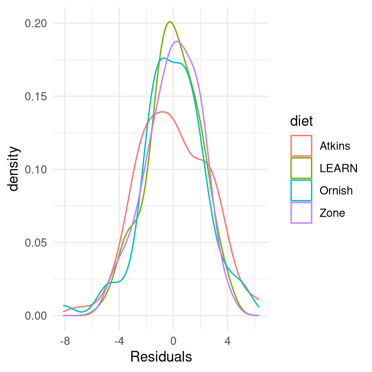
Figure 17.2: Distribution of residuals for for each condition
Another important assumption of the statistical tests that we apply to linear models is that the residuals from the model are normally distributed. It is a common misconception that linear models require that the data are normally distributed, but this is not the case; the only requirement for the statistics to be correct is that the residual errors are normally distributed. The right panel of Figure 17.3 shows a Q-Q (quantile-quantile) plot, which plots the residuals against their expected values based on their quantiles in the normal distribution. If the residuals are normally distributed then the data points should fall along the dashed line — in this case it looks pretty good, except for a couple of outliers that are apparent at the very bottom Because this model is also relatively robust to violations of normality, and these are fairly small, we will go ahead and use the results.
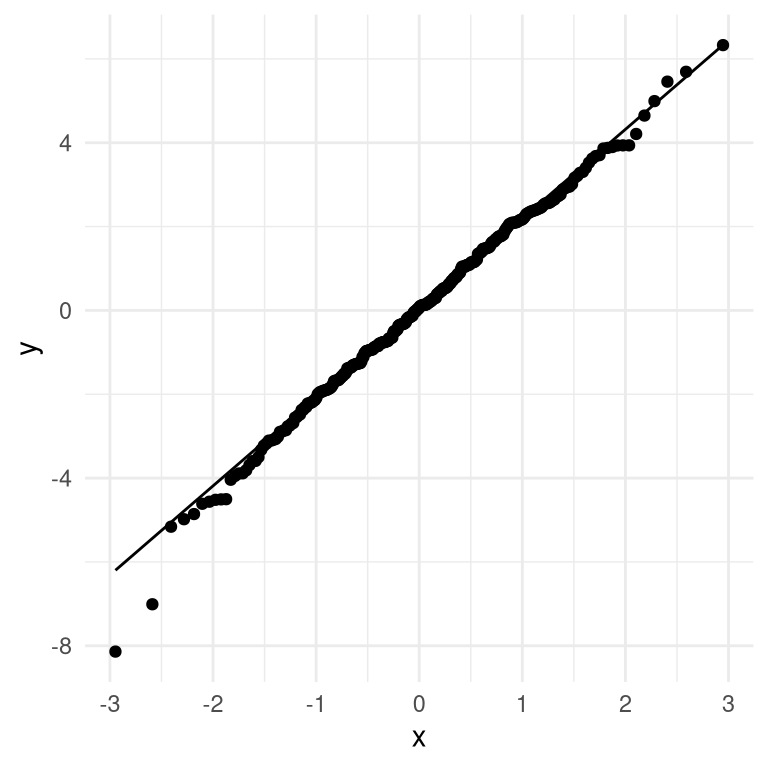
Figure 17.3: Q-Q plot of actual residual values against theoretical residual values
17.1.7 7. Test hypothesis and quantify effect size
First let’s look back at the summary of results from the ANOVA, shown in Step 5 above. The significant F test shows us that there is a significant difference between diets, but we should also note that the model doesn’t actually account for much variance in the data; the R-squared value is only 0.03, showing that the model is only accounting for a few percent of the variance in weight loss. Thus, we would not want to overinterpret this result.
The significant result in the omnibus F test also doesn’t tell us which diets differ from which others. We can find out more by comparing means across conditions. Because we are doing several comparisons, we need to correct for those comparisons, which is accomplished using a procedure known as the Tukey method, which is implemented by our statistical software:
##  diet   emmean    SE  df lower.CL upper.CL .group
##  Atkins  -1.62 0.251 307    -2.11    -1.13  a
##  LEARN   -0.85 0.247 307    -1.34    -0.36  ab
##  Ornish  -0.69 0.252 307    -1.19    -0.19   b
##  Zone    -0.57 0.247 307    -1.06    -0.08   b
##
## Confidence level used: 0.95
## P value adjustment: tukey method for comparing a family of 4 estimates
## significance level used: alpha = 0.05
## NOTE: If two or more means share the same grouping symbol,
##       then we cannot show them to be different.
##       But we also did not show them to be the same.
The letters in the rightmost column show us which of the groups differ from one another, using a method that adjusts for the number of comparisons being performed; conditions that share a letter are not significantly different from one another. This shows that Atkins and LEARN diets don’t differ from one another (since they share the letter a), and the LEARN, Ornish, and Zone diets don’t differ from one another (since they share the letter b), but the Atkins diet differs from the Ornish and Zone diets (since they share no letters).
17.1.8 What about possible confounds?
If we look more closely at the Gardner paper, we will see that they also report statistics on how many individuals in each group had been diagnosed with metabolic syndrome, which is a syndrome characterized by high blood pressure, high blood glucose, excess body fat around the waist, and abnormal cholesterol levels and is associated with increased risk for cardiovascular problems. The data from the Gardner paper are presented in Table 17.1.
| Diet | N | P(metabolic syndrome) |
|---|---|---|
| Atkins | 77 | 0.29 |
| LEARN | 79 | 0.25 |
| Ornish | 76 | 0.38 |
| Zone | 79 | 0.34 |
Looking at the data it seems that the rates are slightly different across groups, with more metabolic syndrome cases in the Ornish and Zone diets – which were exactly the diets with poorer outcomes. Let’s say that we are interested in testing whether the rate of metabolic syndrome was significantly different between the groups, since this might make us concerned that these differences could have affected the results of the diet outcomes.
17.1.8.1 Determine the appropriate model
- What kind of dependent variable?
- proportions
- What are we comparing?
- proportion with metabolic syndrome across four diet groups
- chi-squared test for goodness of fit is appropriate against null hypothesis of no difference
Let’s first compute that statistic, using the chi-squared test function in our statistical software:
##
##  Pearson's Chi-squared test
##
## data:  contTable
## X-squared = 4, df = 3, p-value = 0.3
This test shows that there is not a significant difference between means. However, it doesn’t tell us how certain we are that there is no difference; remember that under NHST, we are always working under the assumption that the null is true unless the data show us enough evidence to cause us to reject the null hypothesis.
What if we want to quantify the evidence for or against the null? We can do this using the Bayes factor.
## Bayes factor analysis
## --------------
## [1] Non-indep. (a=1) : 0.058 ±0%
##
## Against denominator:
##   Null, independence, a = 1
## ---
## Bayes factor type: BFcontingencyTable, independent multinomial
This shows us that the alternative hypothesis is 0.058 times more likely than the null hypothesis, which means that the null hypothesis is 1/0.058 ~ 17 times more likely than the alternative hypothesis given these data. This is fairly strong, if not completely overwhelming, evidence in favor of the null hypothesis.
17.2 Getting help
Whenever one is analyzing real data, it’s useful to check your analysis plan with a trained statistician, as there are many potential problems that could arise in real data. In fact, it’s best to speak to a statistician before you even start the project, as their advice regarding the design or implementation of the study could save you major headaches down the road. Most universities have statistical consulting offices that offer free assistance to members of the university community. Understanding the content of this book won’t prevent you from needing their help at some point, but it will help you have a more informed conversation with them and better understand the advice that they offer.