Chapter 15 Comparing means
We have already encountered a number of cases where we wanted to ask questions about the mean of a sample. In this chapter, we will delve deeper into the various ways that we can compare means across groups.
15.1 Testing the value of a single mean
The simplest question we might want to ask of a mean is whether it has a specific value. Let’s say that we want to test whether the mean diastolic blood pressure value in adults from the NHANES dataset is above 80, which is cutoff for hypertension according to the American College of Cardiology. We take a sample of 200 adults in order to ask this question; each adult had their blood pressure measured three times, and we use the average of these for our test.
One simple way to test for this difference is using a test called the sign test, which asks whether the proportion of positive differences between the actual value and the hypothesized value is different than what we would expect by chance. To do this, we take the differences between each data point and the hypothesized mean value and compute their sign. If the data are normally distributed and the actual mean is equal to the hypothesized mean, then the proportion of values above the hypothesized mean (or below it) should be 0.5, such that the proportion of positive differences should also be 0.5. In our sample, we see that 19.0 percent of individuals have a diastolic blood pressure above 80. We can then use a binomial test to ask whether this proportion of positive differences is greater than 0.5, using the binomial testing function in our statistical software:
##
##  Exact binomial test
##
## data:  npos and nrow(NHANES_sample)
## number of successes = 38, number of trials = 200, p-value = 1
## alternative hypothesis: true probability of success is greater than 0.5
## 95 percent confidence interval:
##  0.15 1.00
## sample estimates:
## probability of success
##                   0.19
Here we see that the proportion of individuals with positive signs is not very surprising under the null hypothesis of \(p \le 0.5\), which should not surprise us given that the observed value is actually less than \(0.5\).
We can also ask this question using Student’s t-test, which you have already encountered earlier in the book. We will refer to the mean as \(\bar{X}\) and the hypothesized population mean as \(\mu\). Then, the t test for a single mean is:
\[ t = \frac{\bar{X} - \mu}{SEM} \] where SEM (as you may remember from the chapter on sampling) is defined as:
\[ SEM = \frac{\hat{\sigma}}{\sqrt{n}} \]
In essence, the t statistic asks how large the deviation of the sample mean from the hypothesized quantity is with respect to the sampling variability of the mean.
We can compute this for the NHANES dataset using our statistical software:
##
##  One Sample t-test
##
## data:  NHANES_adult$BPDiaAve
## t = -55, df = 4593, p-value = 1
## alternative hypothesis: true mean is greater than 80
## 95 percent confidence interval:
##   69 Inf
## sample estimates:
## mean of x
##        70
This shows us that the mean diastolic blood pressure in the dataset (69.5) is actually much lower than 80, so our test for whether it is above 80 is very far from significance.
Remember that a large p-value doesn’t provide us with evidence in favor of the null hypothesis, since we had already assumed that the null hypothesis is true to start with. However, as we discussed in the chapter on Bayesian analysis, we can use the Bayes factor to quantify evidence for or against the null hypothesis:
## Bayes factor analysis
## --------------
## [1] Alt., r=0.707 -Inf<d<80    : 2.7e+16  ±NA%
## [2] Alt., r=0.707 !(-Inf<d<80) : NaNe-Inf ±NA%
##
## Against denominator:
##   Null, mu = 80
## ---
## Bayes factor type: BFoneSample, JZS
The first Bayes factor listed here (\(2.73 * 10^{16}\)) denotes the fact that there is exceedingly strong evidence in favor of the null hypothesis over the alternative.
15.2 Comparing two means
A more common question that often arises in statistics is whether there is a difference between the means of two different groups. Let’s say that we would like to know whether regular marijuana smokers watch more television, which we can also ask using the NHANES dataset. We take a sample of 200 individuals from the dataset and test whether the number of hours of television watching per day is related to regular marijuana use. The left panel of Figure 15.1 shows these data using a violin plot.
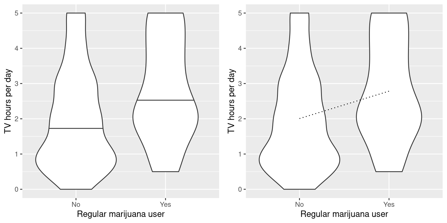
Figure 15.1: Left: Violin plot showing distributions of TV watching separated by regular marijuana use. Right: Violin plots showing data for each group, with a dotted line connecting the predicted values for each group, computed on the basis of the results of the linear model..
We can also use Student’s t test to test for differences between two groups of independent observations (as we saw in an earlier chapter); we will turn later in the chapter to cases where the observations are not independent. As a reminder, the t-statistic for comparison of two independent groups is computed as:
\[ t = \frac{\bar{X_1} - \bar{X_2}}{\sqrt{\frac{S_1^2}{n_1} + \frac{S_2^2}{n_2}}} \]
where \(\bar{X}_1\) and \(\bar{X}_2\) are the means of the two groups, \(S^2_1\) and \(S^2_2\) are the variances for each of the groups, and \(n_1\) and \(n_2\) are the sizes of the two groups. Under the null hypothesis of no difference between means, this statistic is distributed according to a t distribution, with degrees of freedom computed using the Welch test (as discussed previously) since the number of individuals differs between the two groups. In this case, we started with the specific hypothesis that smoking marijuana is associated with greater TV watching, so we will use a one-tailed test. Here are the results from our statistical software:
##
##  Welch Two Sample t-test
##
## data:  TVHrsNum by RegularMarij
## t = -3, df = 85, p-value = 6e-04
## alternative hypothesis: true difference in means between group No and group Yes is less than 0
## 95 percent confidence interval:
##   -Inf -0.39
## sample estimates:
##  mean in group No mean in group Yes
##               2.0               2.8
In this case we see that there is a statistically significant difference between groups, in the expected direction - regular pot smokers watch more TV.
15.3 The t-test as a linear model
The t-test is often presented as a specialized tool for comparing means, but it can also be viewed as an application of the general linear model. In this case, the model would look like this:
\[ \hat{TV} = \hat{\beta_1}*Marijuana + \hat{\beta_0} \] Since smoking is a binary variable, we treat it as a dummy variable like we discussed in the previous chapter, setting it to a value of 1 for smokers and zero for nonsmokers. In that case, \(\hat{\beta_1}\) is simply the difference in means between the two groups, and \(\hat{\beta_0}\) is the mean for the group that was coded as zero. We can fit this model using the general linear model function in our statistical software, and see that it gives the same t statistic as the t-test above, except that it’s positive in this case because of the way that our software arranges the groups:
##
## Call:
## lm(formula = TVHrsNum ~ RegularMarij, data = NHANES_sample)
##
## Residuals:
##     Min      1Q  Median      3Q     Max
## -2.2843 -1.0067 -0.0067  0.9933  2.9933
##
## Coefficients:
##                 Estimate Std. Error t value Pr(>|t|)
## (Intercept)        2.007      0.116   17.27  < 2e-16 ***
## RegularMarijYes    0.778      0.230    3.38  0.00087 ***
## ---
## Signif. codes:  0 '***' 0.001 '**' 0.01 '*' 0.05 '.' 0.1 ' ' 1
##
## Residual standard error: 1.4 on 198 degrees of freedom
## Multiple R-squared:  0.0546, Adjusted R-squared:  0.0498
## F-statistic: 11.4 on 1 and 198 DF,  p-value: 0.000872
We can also view the linear model results graphically (see the right panel of Figure 15.1). In this case, the predicted value for nonsmokers is \(\hat{\beta_0}\) (2.0) and the predicted value for smokers is \(\hat{\beta_0} +\hat{\beta_1}\) (2.8).
To compute the standard errors for this analysis, we can use exactly the same equations that we used for linear regression – since this really is just another example of linear regression. In fact, if you compare the p-value from the t-test above with the p-value in the linear regression analysis for the marijuana use variable, you will see that the one from the linear regression analysis is exactly twice the one from the t-test, because the linear regression analysis is performing a two-tailed test.
15.3.1 Effect sizes for comparing two means
The most commonly used effect size for a comparison between two means is Cohen’s d, which (as you may remember from Chapter 10) is an expression of the effect size in terms of standard deviation units. For the t-test estimated using the general linear model outlined above (i.e. with a single dummy-coded variable), this is expressed as:
\[ d = \frac{\hat{\beta_1}}{\sigma_{residual}} \] We can obtain these values from the analysis output above, giving us a d = 0.55, which we would generally interpret as a medium sized effect.
We can also compute \(R^2\) for this analysis, which tells us what proportion of the variance in TV watching is accounted for by marijuana smoking. This value (which is reported at the bottom of the summary of the linear model analysis above) is 0.05, which tells us that while the effect may be statistically significant, it accounts for relatively little of the variance in TV watching.
15.4 Bayes factor for mean differences
As we discussed in the chapter on Bayesian analysis, Bayes factors provide a way to better quantify evidence in favor of or against the null hypothesis of no difference. We can perform that analysis on the same data:
## Bayes factor analysis
## --------------
## [1] Alt., r=0.707 0<d<Inf    : 0.041 ±0%
## [2] Alt., r=0.707 !(0<d<Inf) : 61    ±0%
##
## Against denominator:
##   Null, mu1-mu2 = 0
## ---
## Bayes factor type: BFindepSample, JZS
Because of the way that the data are organized, the second line shows us the relevant Bayes factor for this analysis, which is 61.4. This shows us that the evidence against the null hypothesis is quite strong.
15.5 Comparing paired observations
In experimental research, we often use within-subjects designs, in which we compare the same person on multiple measurements. The measurements that come from this kind of design are often referred to as repeated measures. For example, in the NHANES dataset blood pressure was measured three times. Let’s say that we are interested in testing whether there is a difference in mean systolic blood pressure between the first and second measurement across individuals in our sample (Figure 15.2).
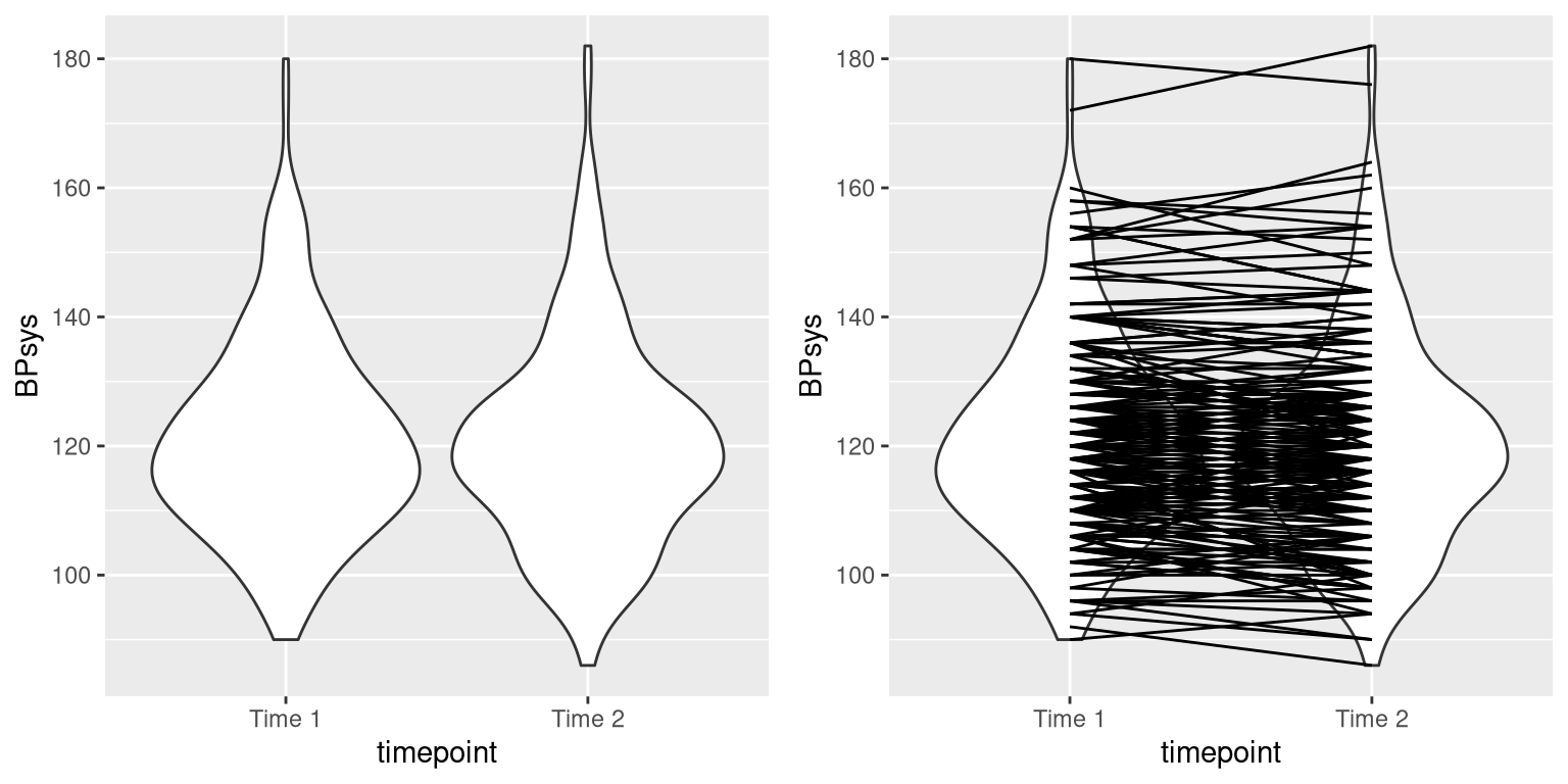
Figure 15.2: Left: Violin plot of systolic blood pressure on first and second recording, from NHANES. Right: Same violin plot with lines connecting the two data points for each individual.
We see that there does not seem to be much of a difference in mean blood pressure (about one point) between the first and second measurement. First let’s test for a difference using an independent samples t-test, which ignores the fact that pairs of data points come from the the same individuals.
##
##  Two Sample t-test
##
## data:  BPsys by timepoint
## t = 0.6, df = 398, p-value = 0.5
## alternative hypothesis: true difference in means between group BPSys1 and group BPSys2 is not equal to 0
## 95 percent confidence interval:
##  -2.1  4.1
## sample estimates:
## mean in group BPSys1 mean in group BPSys2
##                  121                  120
This analysis shows no significant difference. However, this analysis is inappropriate since it assumes that the two samples are independent, when in fact they are not, since the data come from the same individuals. We can plot the data with a line for each individual to show this (see the right panel in Figure 15.2).
In this analysis, what we really care about is whether the blood pressure for each person changed in a systematic way between the two measurements, so another way to represent the data is to compute the difference between the two timepoints for each individual, and then analyze these difference scores rather than analyzing the individual measurements. In Figure 15.3, we show a histogram of these difference scores, with a blue line denoting the mean difference.
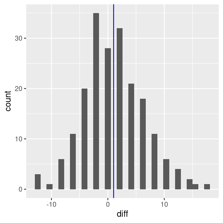
Figure 15.3: Histogram of difference scores between first and second BP measurement. The vertical line represents the mean difference in the sample.
15.5.1 Sign test
One simple way to test for differences is using the sign test. To do this, we take the differences and compute their sign, and then we use a binomial test to ask whether the proportion of positive signs differs from 0.5.
##
##  Exact binomial test
##
## data:  npos and nrow(NHANES_sample)
## number of successes = 96, number of trials = 200, p-value = 0.6
## alternative hypothesis: true probability of success is not equal to 0.5
## 95 percent confidence interval:
##  0.41 0.55
## sample estimates:
## probability of success
##                   0.48
Here we see that the proportion of individuals with positive signs (0.48) is not large enough to be surprising under the null hypothesis of \(p=0.5\). However, one problem with the sign test is that it is throwing away information about the magnitude of the differences, and thus might be missing something.
15.5.2 Paired t-test
A more common strategy is to use a paired t-test, which is equivalent to a one-sample t-test for whether the mean difference between the measurements within each person is zero. We can compute this using our statistical software, telling it that the data points are paired:
##
##  Paired t-test
##
## data:  BPsys by timepoint
## t = 3, df = 199, p-value = 0.007
## alternative hypothesis: true mean difference is not equal to 0
## 95 percent confidence interval:
##  0.29 1.75
## sample estimates:
## mean difference
##               1
With this analyses we see that there is in fact a significant difference between the two measurements. Let’s compute the Bayes factor to see how much evidence is provided by the result:
## Bayes factor analysis
## --------------
## [1] Alt., r=0.707 : 3 ±0.01%
##
## Against denominator:
##   Null, mu = 0
## ---
## Bayes factor type: BFoneSample, JZS
The observed Bayes factor of 2.97 tells us that although the effect was significant in the paired t-test, it actually provides very weak evidence in favor of the alternative hypothesis.
The paired t-test can also be defined in terms of a linear model; see the Appendix for more details on this.
15.6 Comparing more than two means
Often we want to compare more than two means to determine whether any of them differ from one another. Let’s say that we are analyzing data from a clinical trial for the treatment of high blood pressure. In the study, volunteers are randomized to one of three conditions: Drug 1, Drug 2 or placebo. Let’s generate some data and plot them (see Figure 15.4)
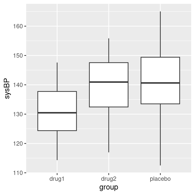
Figure 15.4: Box plots showing blood pressure for three different groups in our clinical trial.
15.6.1 Analysis of variance
We would first like to test the null hypothesis that the means of all of the groups are equal – that is, neither of the treatments had any effect compared to placebo. We can do this using a method called analysis of variance (ANOVA). This is one of the most commonly used methods in psychological statistics, and we will only scratch the surface here. The basic idea behind ANOVA is one that we already discussed in the chapter on the general linear model, and in fact ANOVA is just a name for a specific version of such a model.
Remember from the last chapter that we can partition the total variance in the data (\(SS_{total}\)) into the variance that is explained by the model (\(SS_{model}\)) and the variance that is not (\(SS_{error}\)). We can then compute a mean square for each of these by dividing them by their degrees of freedom; for the error this is \(N - p\) (where \(p\) is the number of means that we have computed), and for the model this is \(p - 1\):
\[ MS_{model} =\frac{SS_{model}}{df_{model}}= \frac{SS_{model}}{p-1} \]
\[ MS_{error} = \frac{SS_{error}}{df_{error}} = \frac{SS_{error}}{N - p} \]
With ANOVA, we want to test whether the variance accounted for by the model is greater than what we would expect by chance, under the null hypothesis of no differences between means. Whereas for the t distribution the expected value is zero under the null hypothesis, that’s not the case here, since sums of squares are always positive numbers. Fortunately, there is another theoretical distribution that describes how ratios of sums of squares are distributed under the null hypothesis: The F distribution (see figure 15.5). This distribution has two degrees of freedom, which correspond to the degrees of freedom for the numerator (which in this case is the model), and the denominator (which in this case is the error).
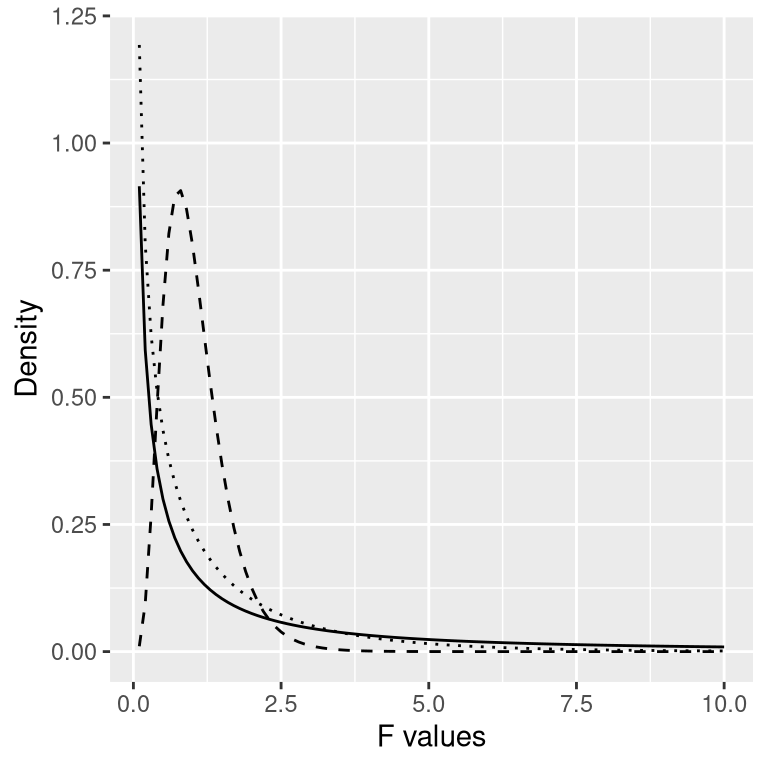
Figure 15.5: F distributions under the null hypothesis, for different values of degrees of freedom.
To create an ANOVA model, we extend the idea of dummy coding that you encountered in the last chapter. Remember that for the t-test comparing two means, we created a single dummy variable that took the value of 1 for one of the conditions and zero for the others. Here we extend that idea by creating two dummy variables, one that codes for the Drug 1 condition and the other that codes for the Drug 2 condition. Just as in the t-test, we will have one condition (in this case, placebo) that doesn’t have a dummy variable, and thus represents the baseline against which the others are compared; its mean defines the intercept of the model. Using dummy coding for drugs 1 and 2, we can fit a model using the same approach that we used in the previous chapter:
##
## Call:
## lm(formula = sysBP ~ d1 + d2, data = df)
##
## Residuals:
##     Min      1Q  Median      3Q     Max
## -29.084  -7.745  -0.098   7.687  23.431
##
## Coefficients:
##             Estimate Std. Error t value Pr(>|t|)
## (Intercept)   141.60       1.66   85.50  < 2e-16 ***
## d1            -10.24       2.34   -4.37  2.9e-05 ***
## d2             -2.03       2.34   -0.87     0.39
## ---
## Signif. codes:  0 '***' 0.001 '**' 0.01 '*' 0.05 '.' 0.1 ' ' 1
##
## Residual standard error: 9.9 on 105 degrees of freedom
## Multiple R-squared:  0.169,  Adjusted R-squared:  0.154
## F-statistic: 10.7 on 2 and 105 DF,  p-value: 5.83e-05
The output from this command provides us with two things. First, it shows us the result of a t-test for each of the dummy variables, which basically tell us whether each of the conditions separately differs from placebo; it appears that Drug 1 does whereas Drug 2 does not. However, keep in mind that if we wanted to interpret these tests, we would need to correct the p-values to account for the fact that we have done multiple hypothesis tests; we will see an example of how to do this in the next chapter.
Remember that the hypothesis that we started out wanting to test was whether there was any difference between any of the conditions; we refer to this as an omnibus hypothesis test, and it is the test that is provided by the F statistic. The F statistic basically tells us whether our model is better than a simple model that just includes an intercept. In this case we see that the F test is highly significant, consistent with our impression that there did seem to be differences between the groups (which in fact we know there were, because we created the data).
15.7 Learning objectives
After reading this chapter, you should be able to:
- Describe the rationale behind the sign test
- Describe how the t-test can be used to compare a single mean to a hypothesized value
- Compare the means for two paired or unpaired groups using a two-sample t-test
- Describe how analysis of variance can be used to test differences between more than two means.
15.8 Appendix
15.8.1 The paired t-test as a linear model
We can also define the paired t-test in terms of a general linear model. To do this, we include all of the measurements for each subject as data points (within a tidy data frame). We then include in the model a variable that codes for the identity of each individual (in this case, the ID variable that contains a subject ID for each person). This is known as a mixed model, since it includes effects of independent variables as well as effects of individuals. The standard model fitting procedure lm() can’t do this, but we can do it using the lmer() function from a popular R package called lme4, which is specialized for estimating mixed models. The (1|ID) in the formula tells lmer() to estimate a separate intercept (which is what the 1 refers to) for each value of the ID variable (i.e. for each individual in the dataset), and then estimate a common slope relating timepoint to BP.
# compute mixed model for paired test

lmrResult <- lmer(BPsys ~ timepoint + (1 | ID),
                  data = NHANES_sample_tidy)
summary(lmrResult)
## Linear mixed model fit by REML. t-tests use Satterthwaite's method [
## lmerModLmerTest]
## Formula: BPsys ~ timepoint + (1 | ID)
## Data: NHANES_sample_tidy
##
## REML criterion at convergence: 2895
##
## Scaled residuals:
## Min 1Q Median 3Q Max
## -2.3843 -0.4808 0.0076 0.4221 2.1718
##
## Random effects:
## Groups Name Variance Std.Dev.
## ID (Intercept) 236.1 15.37
## Residual 13.9 3.73
## Number of obs: 400, groups: ID, 200
##
## Fixed effects:
## Estimate Std. Error df t value Pr(>|t|)
## (Intercept) 121.370 1.118 210.361 108.55 <2e-16 ***
## timepointBPSys2 -1.020 0.373 199.000 -2.74 0.0068 **
## ---
## Signif. codes: 0 '***' 0.001 '**' 0.01 '*' 0.05 '.' 0.1 ' ' 1
##
## Correlation of Fixed Effects:
## (Intr)
## tmpntBPSys2 -0.167You can see that this shows us a p-value that is very close to the result from the paired t-test computed using the t.test() function.