Chapter 6 Probability
Probability theory is the branch of mathematics that deals with chance and uncertainty. It forms an important part of the foundation for statistics, because it provides us with the mathematical tools to describe uncertain events. The study of probability arose in part due to interest in understanding games of chance, like cards or dice. These games provide useful examples of many statistical concepts, because when we repeat these games the likelihood of different outcomes remains (mostly) the same. However, there are deep questions about the meaning of probability that we will not address here; see Suggested Readings at the end if you are interested in learning more about this fascinating topic and its history.
6.1 What is probability?
Informally, we usually think of probability as a number that describes the likelihood of some event occurring, which ranges from zero (impossibility) to one (certainty). Sometimes probabilities will instead be expressed in percentages, which range from zero to one hundred, as when the weather forecast predicts a twenty percent chance of rain today. In each case, these numbers are expressing how likely that particular event is, ranging from absolutely impossible to absolutely certain.
To formalize probability theory, we first need to define a few terms:
- An experiment is any activity that produces or observes an outcome. Examples are flipping a coin, rolling a 6-sided die, or trying a new route to work to see if it’s faster than the old route.
- The sample space is the set of possible outcomes for an experiment. We represent these by listing them within a set of squiggly brackets. For a coin flip, the sample space is {heads, tails}. For a six-sided die, the sample space is each of the possible numbers that can appear: {1,2,3,4,5,6}. For the amount of time it takes to get to work, the sample space is all possible real numbers greater than zero (since it can’t take a negative amount of time to get somewhere, at least not yet). We won’t bother trying to write out all of those numbers within the brackets.
- An event is a subset of the sample space. In principle it could be one or more of possible outcomes in the sample space, but here we will focus primarily on elementary events which consist of exactly one possible outcome. For example, this could be obtaining heads in a single coin flip, rolling a 4 on a throw of the die, or taking 21 minutes to get home by the new route.
Now that we have those definitions, we can outline the formal features of a probability, which were first defined by the Russian mathematician Andrei Kolmogorov. These are the features that a value has to have if it is going to be a probability. Let’s say that we have a sample space defined by N independent events, \({E_1, E_2, ... , E_N}\), and \(X\) is a random variable denoting which of the events has occurred. \(P(X=E_i)\) is the probability of event \(i\):
- Probability cannot be negative: \(P(X=E_i) \ge 0\)
- The total probability of all outcomes in the sample space is 1; that is, if the , if we take the probability of each Ei and add them up, they must sum to 1. We can express this using the summation symbol \(\sum\):
\[
\sum_{i=1}^N{P(X=E_i)} = P(X=E_1) + P(X=E_2) + ... + P(X=E_N) = 1
\]
This is interpreted as saying “Take all of the N elementary events, which we have labeled from 1 to N, and add up their probabilities. These must sum to one.”
- The probability of any individual event cannot be greater than one: \(P(X=E_i)\le 1\). This is implied by the previous point; since they must sum to one, and they can’t be negative, then any particular probability cannot exceed one.
6.2 How do we determine probabilities?
Now that we know what a probability is, how do we actually figure out what the probability is for any particular event?
6.2.1 Personal belief
Let’s say that I asked you what the probability was that Bernie Sanders would have won the 2016 presidential election if he had been the democratic nominee instead of Hilary Clinton? We can’t actually do the experiment to find the outcome. However, most people with knowledge of American politics would be willing to at least offer a guess at the probability of this event. In many cases personal knowledge and/or opinion is the only guide we have determining the probability of an event, but this is not very scientifically satisfying.
6.2.2 Empirical frequency
Another way to determine the probability of an event is to do the experiment many times and count how often each event happens. From the relative frequency of the different outcomes, we can compute the probability of each outcome. For example, let’s say that we are interested in knowing the probability of rain in San Francisco. We first have to define the experiment — let’s say that we will look at the National Weather Service data for each day in 2017 and determine whether there was any rain at the downtown San Francisco weather station. According to these data, in 2017 there were 73 rainy days. To compute the probability of rain in San Francisco, we simply divide the number of rainy days by the number of days counted (365), giving P(rain in SF in 2017) = 0.2.
How do we know that empirical probability gives us the right number? The answer to this question comes from the law of large numbers, which shows that the empirical probability will approach the true probability as the sample size increases. We can see this by simulating a large number of coin flips, and looking at our estimate of the probability of heads after each flip. We will spend more time discussing simulation in a later chapter; for now, just assume that we have a computational way to generate a random outcome for each coin flip.
The left panel of Figure 6.1 shows that as the number of samples (i.e., coin flip trials) increases, the estimated probability of heads converges onto the true value of 0.5. However, note that the estimates can be very far off from the true value when the sample sizes are small. A real-world example of this was seen in the 2017 special election for the US Senate in Alabama, which pitted the Republican Roy Moore against Democrat Doug Jones. The right panel of Figure 6.1 shows the relative amount of the vote reported for each of the candidates over the course of the evening, as an increasing number of ballots were counted. Early in the evening the vote counts were especially volatile, swinging from a large initial lead for Jones to a long period where Moore had the lead, until finally Jones took the lead to win the race.
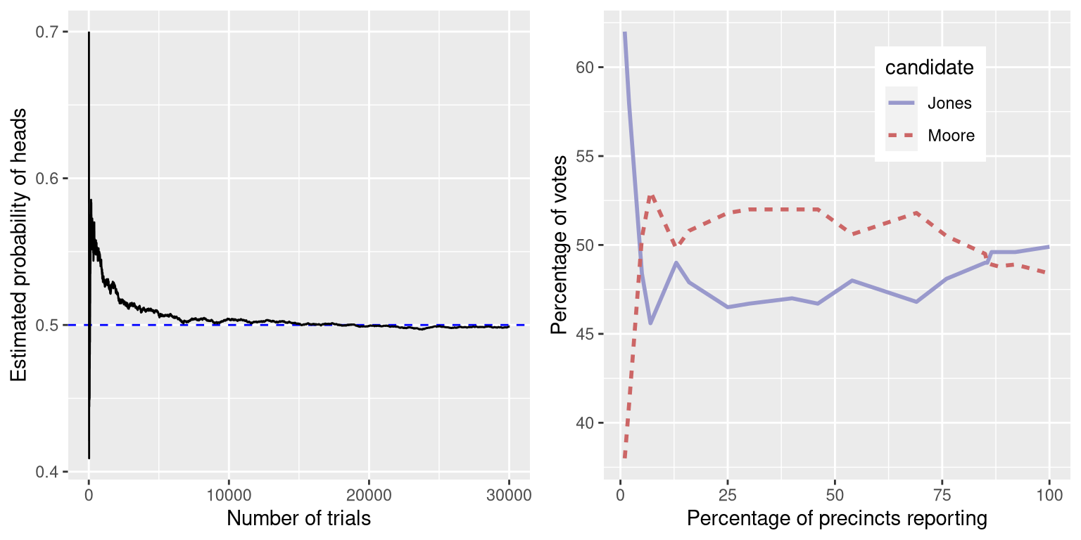
Figure 6.1: Left: A demonstration of the law of large numbers. A coin was flipped 30,000 times, and after each flip the probability of heads was computed based on the number of heads and tail collected up to that point. It takes about 15,000 flips for the probability to settle at the true probability of 0.5. Right: Relative proportion of the vote in the Dec 12, 2017 special election for the US Senate seat in Alabama, as a function of the percentage of precincts reporting. These data were transcribed from https://www.ajc.com/news/national/alabama-senate-race-live-updates-roy-moore-doug-jones/KPRfkdaweoiXICW3FHjXqI/
These two examples show that while large samples will ultimately converge on the true probability, the results with small samples can be far off. Unfortunately, many people forget this and overinterpret results from small samples. This was referred to as the law of small numbers by the psychologists Danny Kahneman and Amos Tversky, who showed that people (even trained researchers) often behave as if the law of large numbers applies even to small samples, giving too much credence to results based on small datasets. We will see examples throughout the course of just how unstable statistical results can be when they are generated on the basis of small samples.
6.2.3 Classical probability
It’s unlikely that any of us has ever flipped a coin tens of thousands of times, but we are nonetheless willing to believe that the probability of flipping heads is 0.5. This reflects the use of yet another approach to computing probabilities, which we refer to as classical probability. In this approach, we compute the probability directly based on our knowledge of the situation.
Classical probability arose from the study of games of chance such as dice and cards. A famous example arose from a problem encountered by a French gambler who went by the name of Chevalier de Méré. de Méré played two different dice games: In the first he bet on the chance of at least one six on four rolls of a six-sided die, while in the second he bet on the chance of at least one double-six on 24 rolls of two dice. He expected to win money on both of these gambles, but he found that while on average he won money on the first gamble, he actually lost money on average when he played the second gamble many times. To understand this he turned to his friend, the mathematician Blaise Pascal, who is now recognized as one of the founders of probability theory.
How can we understand this question using probability theory? In classical probability, we start with the assumption that all of the elementary events in the sample space are equally likely; that is, when you roll a die, each of the possible outcomes ({1,2,3,4,5,6}) is equally likely to occur. (No loaded dice allowed!) Given this, we can compute the probability of any individual outcome as one divided by the number of possible outcomes:
\[ P(outcome_i) = \frac{1}{\text{number of possible outcomes}} \]
For the six-sided die, the probability of each individual outcome is 1/6.
This is nice, but de Méré was interested in more complex events, like what happens on multiple dice throws. How do we compute the probability of a complex event (which is a union of single events), like rolling a six on the first or the second throw? We represent the union of events mathematically using the \(\cup\) symbol: for example, if the probability of rolling a six on the first throw is referred to as \(P(Roll6_{throw1})\) and the probability of rolling a six on the second throw is \(P(Roll6_{throw2})\), then the union is referred to as \(P(Roll6_{throw1} \cup Roll6_{throw2})\).
de Méré thought (incorrectly, as we will see below) that he could simply add together the probabilities of the individual events to compute the probability of the combined event, meaning that the probability of rolling a six on the first or second roll would be computed as follows:
\[ P(Roll6_{throw1}) = 1/6 \] \[ P(Roll6_{throw2}) = 1/6 \]
\[ de Méré's \ error: \] \[ P(Roll6_{throw1} \cup Roll6_{throw2}) = P(Roll6_{throw1}) + P(Roll6_{throw2}) = 1/6 + 1/6 = 1/3 \]
de Méré reasoned based on this incorrect assumption that the probability of at least one six in four rolls was the sum of the probabilities on each of the individual throws: \(4*\frac{1}{6}=\frac{2}{3}\). Similarly, he reasoned that since the probability of a double-six when throwing two dice is 1/36, then the probability of at least one double-six on 24 rolls of two dice would be \(24*\frac{1}{36}=\frac{2}{3}\). Yet, while he consistently won money on the first bet, he lost money on the second bet. What gives?
To understand de Méré’s error, we need to introduce some of the rules of probability theory. The first is the rule of subtraction, which says that the probability of some event A not happening is one minus the probability of the event happening:
\[ P(\neg A) = 1 - P(A) \]
where \(\neg A\) means “not A”. This rule derives directly from the axioms that we discussed above; because A and \(\neg A\) are the only possible outcomes, then their total probability must sum to 1. For example, if the probability of rolling a one in a single throw is \(\frac{1}{6}\), then the probability of rolling anything other than a one is \(\frac{5}{6}\).
A second rule tells us how to compute the probability of a conjoint event – that is, the probability that both of two events will occur. We refer to this as an intersection, which is signified by the \(\cap\) symbol; thus, \(P(A \cap B)\) means the probability that both A and B will occur. We will focus on a version of the rule that tells us how to compute this quantity in the special case when the two events are independent from one another; we will learn later exactly what the concept of independence means, but for now we can just take it for granted that the two die throws are independent events. We compute the probability of the intersection of two independent events by simply multiplying the probabilities of the individual events:
\[ P(A \cap B) = P(A) * P(B)\ \text{if and only if A and B are independent} \] Thus, the probability of throwing a six on both of two rolls is \(\frac{1}{6}*\frac{1}{6}=\frac{1}{36}\).
The third rule tells us how to add together probabilities - and it is here that we see the source of de Méré’s error. The addition rule tells us that to obtain the probability of either of two events occurring, we add together the individual probabilities, but then subtract the likelihood of both occurring together:
\[ P(A \cup B) = P(A) + P(B) - P(A \cap B) \] In a sense, this prevents us from counting those instances twice, and that’s what distinguishes the rule from de Méré’s incorrect computation. Let’s say that we want to find the probability of rolling 6 on either of two throws. According to our rules:
\[ P(Roll6_{throw1} \cup Roll6_{throw2}) = P(Roll6_{throw1}) + P(Roll6_{throw2}) - P(Roll6_{throw1} \cap Roll6_{throw2}) \] \[ = \frac{1}{6} + \frac{1}{6} - \frac{1}{36} = \frac{11}{36} \]
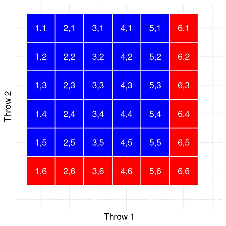
Figure 6.2: Each cell in this matrix represents one outcome of two throws of a die, with the columns representing the first throw and the rows representing the second throw. Cells shown in red represent the cells with a six in either the first or second throw; the rest are shown in blue.
Let’s use a graphical depiction to get a different view of this rule. Figure 6.2 shows a matrix representing all possible combinations of results across two throws, and highlights the cells that involve a six on either the first or second throw. If you count up the cells in red you will see that there are 11 such cells. This shows why the addition rule gives a different answer from de Méré’s; if we were to simply add together the probabilities for the two throws as he did, then we would count (6,6) towards both, when it should really only be counted once.
6.2.4 Solving de Méré’s problem
Blaise Pascal used the rules of probability to come up with a solution to de Méré’s problem. First, he realized that computing the probability of at least one event out of a combination was tricky, whereas computing the probability that something does not occur across several events is relatively easy – it’s just the product of the probabilities of the individual events. Thus, rather than computing the probability of at least one six in four rolls, he instead computed the probability of no sixes across all rolls:
\[ P(\text{no sixes in four rolls}) = \frac{5}{6}*\frac{5}{6}*\frac{5}{6}*\frac{5}{6}=\bigg(\frac{5}{6}\bigg)^4=0.482 \]
He then used the fact that the probability of no sixes in four rolls is the complement of at least one six in four rolls (thus they must sum to one), and used the rule of subtraction to compute the probability of interest:
\[ P(\text{at least one six in four rolls}) = 1 - \bigg(\frac{5}{6}\bigg)^4=0.517 \]
de Méré’s gamble that he would throw at least one six in four rolls has a probability of greater than 0.5, explaning why de Méré made money on this bet on average.
But what about de Méré’s second bet? Pascal used the same trick:
\[ P(\text{no double six in 24 rolls}) = \bigg(\frac{35}{36}\bigg)^{24}=0.509 \] \[ P(\text{at least one double six in 24 rolls}) = 1 - \bigg(\frac{35}{36}\bigg)^{24}=0.491 \]
The probability of this outcome was slightly below 0.5, showing why de Méré lost money on average on this bet.
6.3 Probability distributions
A probability distribution describes the probability of all of the possible outcomes in an experiment. For example, on Jan 20 2018, the basketball player Steph Curry hit only 2 out of 4 free throws in a game against the Houston Rockets. We know that Curry’s overall probability of hitting free throws across the entire season was 0.91, so it seems pretty unlikely that he would hit only 50% of his free throws in a game, but exactly how unlikely is it? We can determine this using a theoretical probability distribution; throughout this book we will encounter a number of these probability distributions, each of which is appropriate to describe different types of data. In this case, we use the binomial distribution, which provides a way to compute the probability of some number of successes out of a number of trials on which there is either success or failure and nothing in between (known as “Bernoulli trials”), given some known probability of success on each trial. This distribution is defined as:
\[ P(k; n,p) = P(X=k) = \binom{n}{k} p^k(1-p)^{n-k} \]
This refers to the probability of k successes on n trials when the probability of success is p. You may not be familiar with \(\binom{n}{k}\), which is referred to as the binomial coefficient. The binomial coefficient is also referred to as “n-choose-k” because it describes the number of different ways that one can choose k items out of n total items. The binomial coefficient is computed as:
\[ \binom{n}{k} = \frac{n!}{k!(n-k)!} \] where the exclamation point (!) refers to the factorial of the number:
\[ n! = \prod_{i=1}^n i = n*(n-1)*...*2*1 \]
The product operator \(\prod\) is similar to the summation operator \(\sum\), except that it multiplies instead of adds. In this case, it is multiplying together all numbers from one to \(n\).
In the example of Steph Curry’s free throws:
\[ P(2;4,0.91) = \binom{4}{2} 0.91^2(1-0.91)^{4-2} = 0.040 \]
This shows that given Curry’s overall free throw percentage, it is very unlikely that he would hit only 2 out of 4 free throws. Which just goes to show that unlikely things do actually happen in the real world.
6.3.1 Cumulative probability distributions
Often we want to know not just how likely a specific value is, but how likely it is to find a value that is as extreme or more than a particular value; this will become very important when we discuss hypothesis testing in Chapter 9. To answer this question, we can use a cumulative probability distribution; whereas a standard probability distribution tells us the probability of some specific value, the cumulative distribution tells us the probability of a value as large or larger (or as small or smaller) than some specific value.
In the free throw example, we might want to know: What is the probability that Steph Curry hits 2 or fewer free throws out of four, given his overall free throw probability of 0.91. To determine this, we could simply use the the binomial probability equation and plug in all of the possible values of k and add them together:
\[ P(k\le2)= P(k=2) + P(k=1) + P(k=0) = 6e^{-5} + .002 + .040 = .043 \]
In many cases the number of possible outcomes would be too large for us to compute the cumulative probability by enumerating all possible values; fortunately, it can be computed directly for any theoretical probability distribution. Table 6.1 shows the cumulative probability of each possible number of successful free throws in the example from above, from which we can see that the probability of Curry landing 2 or fewer free throws out of 4 attempts is 0.043.
| numSuccesses | Probability | CumulativeProbability |
|---|---|---|
| 0 | 0.000 | 0.000 |
| 1 | 0.003 | 0.003 |
| 2 | 0.040 | 0.043 |
| 3 | 0.271 | 0.314 |
| 4 | 0.686 | 1.000 |
6.4 Conditional probability
So far we have limited ourselves to simple probabilities - that is, the probability of a single event or combination of events. However, we often wish to determine the probability of some event given that some other event has occurred, which are known as conditional probabilities.
Let’s take the 2016 US Presidential election as an example. There are two simple probabilities that we could use to describe the electorate. First, we know the probability that a voter in the US is affiliated with the Republican party: \(p(Republican) = 0.44\). We also know the probability that a voter cast their vote in favor of Donald Trump: \(p(Trump voter)=0.46\). However, let’s say that we want to know the following: What is the probability that a person cast their vote for Donald Trump, given that they are a Republican?
To compute the conditional probability of A given B (which we write as \(P(A|B)\), “probability of A, given B”), we need to know the joint probability (that is, the probability of both A and B occurring) as well as the overall probability of B:
\[ P(A|B) = \frac{P(A \cap B)}{P(B)} \]
That is, we want to know the probability that both things are true, given that the one being conditioned upon is true.
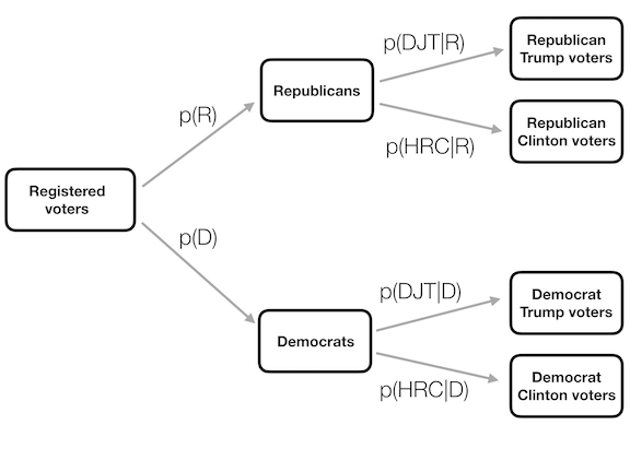
Figure 6.3: A graphical depiction of conditional probability, showing how the conditional probability limits our analysis to a subset of the data.
It can be useful to think of this graphically. Figure 6.3 shows a flow chart depicting how the full population of voters breaks down into Republicans and Democrats, and how the conditional probability (conditioning on party) further breaks down the members of each party according to their vote.
6.5 Computing conditional probabilities from data
We can also compute conditional probabilities directly from data. Let’s say that we are interested in the following question: What is the probability that someone has diabetes, given that they are not physically active? – that is, \(P(diabetes|inactive)\). The NHANES dataset includes two variables that address the two parts of this question. The first (Diabetes) asks whether the person has ever been told that they have diabetes, and the second (PhysActive) records whether the person engages in sports, fitness, or recreational activities that are at least of moderate intensity. Let’s first compute the simple probabilities, which are shown in Table 6.2. The table shows that the probability that someone in the NHANES dataset has diabetes is .1, and the probability that someone is inactive is .45.
| Answer | N_diabetes | P_diabetes | N_PhysActive | P_PhysActive |
|---|---|---|---|---|
| No | 4893 | 0.9 | 2472 | 0.45 |
| Yes | 550 | 0.1 | 2971 | 0.55 |
| Diabetes | PhysActive | n | prob |
|---|---|---|---|
| No | No | 2123 | 0.39 |
| No | Yes | 2770 | 0.51 |
| Yes | No | 349 | 0.06 |
| Yes | Yes | 201 | 0.04 |
To compute \(P(diabetes|inactive)\) we would also need to know the joint probability of being diabetic and inactive, in addition to the simple probabilities of each. These are shown in Table 6.3. Based on these joint probabilities, we can compute \(P(diabetes|inactive)\). One way to do this in a computer program is to first determine the whether the PhysActive variable was equal to “No” for each indivdual, and then take the mean of those truth values. Since TRUE/FALSE values are treated as 1/0 respectively by most programming languages (including R and Python), this allows us to easily identify the probability of a simple event by simply taking the mean of a logical variable representing its truth value. We then use that value to compute the conditional probability, where we find that the probability of someone having diabetes given that they are physically inactive is 0.141.
6.6 Independence
The term “independent” has a very specific meaning in statistics, which is somewhat different from the common usage of the term. Statistical independence between two variables means that knowing the value of one variable doesn’t tell us anything about the value of the other. This can be expressed as:
\[ P(A|B) = P(A) \]
That is, the probability of A given some value of B is just the same as the overall probability of A. Looking at it this way, we see that many cases of what we would call “independence” in the real world are not actually statistically independent. For example, there is currently a move by a small group of California citizens to declare a new independent state called Jefferson, which would comprise a number of counties in northern California and Oregon. If this were to happen, then the probability that a current California resident would now live in the state of Jefferson would be \(P(\text{Jeffersonian})=0.014\), whereas the probability that they would remain a California resident would be \(P(\text{Californian})=0.986\). The new states might be politically independent, but they would not be statistically independent, because if we know that a person is Jeffersonian, then we can be sure that they are not Californian! That is, while independence in common language often refers to sets that are exclusive, statistical independence refers to the case where one cannot predict anything about one variable from the value of another variable. For example, knowing a person’s hair color is unlikely to tell you whether they prefer chocolate or strawberry ice cream.
Let’s look at another example, using the NHANES data: Are physical health and mental health independent of one another? NHANES includes two relevant questions: PhysActive, which asks whether the individual is physically active, and DaysMentHlthBad, which asks how many days out of the last 30 that the individual experienced bad mental health. Let’s consider anyone who had more than 7 days of bad mental health in the last month to be in bad mental health. Based on this, we can define a new variable called badMentalHealth as a logical variable telling whether each person had more than 7 days of bad mental health or not. We can first summarize the data to show how many individuals fall into each combination of the two variables (shown in Table 6.4), and then divide by the total number of observations to create a table of proportions (shown in Table 6.5):
| PhysActive | Bad Mental Health | Good Mental Health | Total |
|---|---|---|---|
| No | 414 | 1664 | 2078 |
| Yes | 292 | 1926 | 2218 |
| Total | 706 | 3590 | 4296 |
| PhysActive | Bad Mental Health | Good Mental Health | Total |
|---|---|---|---|
| No | 0.10 | 0.39 | 0.48 |
| Yes | 0.07 | 0.45 | 0.52 |
| Total | 0.16 | 0.84 | 1.00 |
This shows us the proportion of all observations that fall into each cell. However, what we want to know here is the conditional probability of bad mental health, depending on whether one is physically active or not. To compute this, we divide each physical activity group by its total number of observations, so that each row now sums to one (shown in Table 6.6). Here we see the conditional probabilities of bad or good mental health for each physical activity group (in the top two rows) along with the overall probability of good or bad mental health in the third row. To determine whether mental health and physical activity are independent, we would compare the simple probability of bad mental health (in the third row) to the conditional probability of bad mental health given that one is physically active (in the second row).
| PhysActive | Bad Mental Health | Good Mental Health | Total |
|---|---|---|---|
| No | 0.20 | 0.80 | 1 |
| Yes | 0.13 | 0.87 | 1 |
| Total | 0.16 | 0.84 | 1 |
The overall probability of bad mental health \(P(\text{bad mental health})\) is 0.16 while the conditional probability \(P(\text{bad mental health|physically active})\) is 0.13. Thus, it seems that the conditional probability is somewhat smaller than the overall probability, suggesting that they are not independent, though we can’t know for sure just by looking at the numbers, since these numbers might be different due to random variability in our sample. Later in the book we will discuss statistical tools that will let us directly test whether two variables are independent.
6.7 Reversing a conditional probability: Bayes’ rule
In many cases, we know \(P(A|B)\) but we really want to know \(P(B|A)\). This commonly occurs in medical screening, where we know \(P(\text{positive test result| disease})\) but what we want to know is \(P(\text{disease|positive test result})\). For example, some doctors recommend that men over the age of 50 undergo screening using a test called prostate specific antigen (PSA) to screen for possible prostate cancer. Before a test is approved for use in medical practice, the manufacturer needs to test two aspects of the test’s performance. First, they need to show how sensitive it is – that is, how likely is it to find the disease when it is present: \(\text{sensitivity} = P(\text{positive test| disease})\). They also need to show how specific it is: that is, how likely is it to give a negative result when there is no disease present: \(\text{specificity} = P(\text{negative test|no disease})\). For the PSA test, we know that sensitivity is about 80% and specificity is about 70%. However, these don’t answer the question that the physician wants to answer for any particular patient: what is the likelihood that they actually have cancer, given that the test comes back positive? This requires that we reverse the conditional probability that defines sensitivity: instead of \(P(positive\ test| disease)\) we want to know \(P(disease|positive\ test)\).
In order to reverse a conditional probability, we can use Bayes’ rule:
\[ P(B|A) = \frac{P(A|B)*P(B)}{P(A)} \]
Bayes’ rule is fairly easy to derive, based on the rules of probability that we learned earlier in the chapter (see the Appendix for this derivation).
If we have only two outcomes, we can express Bayes’ rule in a somewhat clearer way, using the sum rule to redefine \(P(A)\):
\[ P(A) = P(A|B)*P(B) + P(A|\neg B)*P(\neg B) \]
Using this, we can redefine Bayes’s rule:
\[ P(B|A) = \frac{P(A|B)*P(B)}{P(A|B)*P(B) + P(A|\neg B)*P(\neg B)} \]
We can plug the relevant numbers into this equation to determine the likelihood that an individual with a positive PSA result actually has cancer – but note that in order to do this, we also need to know the overall probability of cancer for that person, which we often refer to as the base rate. Let’s take a 60 year old man, for whom the probability of prostate cancer in the next 10 years is \(P(cancer)=0.058\). Using the sensitivity and specificity values that we outlined above, we can compute the individual’s likelihood of having cancer given a positive test:
\[ P(\text{cancer|test}) = \frac{P(\text{test|cancer})*P(\text{cancer})}{P(\text{test|cancer})*P(\text{cancer}) + P(\text{test|}\neg\text{cancer})*P(\neg\text{cancer})} \] \[ = \frac{0.8*0.058}{0.8*0.058 +0.3*0.942 } = 0.14 \] That’s pretty small – do you find that surprising? Many people do, and in fact there is a substantial psychological literature showing that people systematically neglect base rates (i.e. overall prevalence) in their judgments.
6.8 Learning from data
Another way to think of Bayes’ rule is as a way to update our beliefs on the basis of data – that is, learning about the world using data. Let’s look at Bayes’ rule again:
\[ P(B|A) = \frac{P(A|B)*P(B)}{P(A)} \]
The different parts of Bayes’ rule have specific names, that relate to their role in using Bayes’ rule to update our beliefs. We start out with an initial guess about the probability of B (\(P(B)\)), which we refer to as the prior probability. In the PSA example we used the base rate as our prior, since it was our best guess as to the individual’s chance of cancer before we knew the test result. We then collect some data, which in our example was the test result. The degree to which the data A are consistent with outcome B is given by \(P(A|B)\), which we refer to as the likelihood. You can think of this as how likely the data are, given that the particular hypothesis being tested is true. In our example, the hypothesis being tested was whether the individual had cancer, and the likelihood was based on our knowledge about the sensitivity of the test (that is, the probability of a positive test outcome given cancer is present). The denominator (\(P(A)\)) is referred to as the marginal likelihood, because it expresses the overall likelihood of the data, averaged across all of the possible values of B (which in our example were disease present and disease absent). The outcome to the left (\(P(B|A)\)) is referred to as the posterior - because it’s what comes out the back end of the computation.
There is another way of writing Bayes rule that makes this a bit clearer:
\[ P(B|A) = \frac{P(A|B)}{P(A)}*P(B) \]
The part on the left (\(\frac{P(A|B)}{P(A)}\)) tells us how much more or less likely the data A are given B, relative to the overall (marginal) likelihood of the data, while the part on the right side (\(P(B)\)) tells us how likely we thought B was before we knew anything about the data. This makes it clearer that the role of Bayes theorem is to update our prior knowledge based on the degree to which the data are more likely given B than they would be overall. If the hypothesis is more likely given the data than it would be in general, then we increase our belief in the hypothesis; if it’s less likely given the data, then we decrease our belief.
6.9 Odds and odds ratios
The result in the last section showed that the likelihood that the individual has cancer based on a positive PSA test result is still fairly low, even though it’s more than twice as big as it was before we knew the test result. We would often like to quantify the relation between probabilities more directly, which we can do by converting them into odds which express the relative likelihood of something happening or not:
\[
\text{odds of A} = \frac{P(A)}{P(\neg A)}
\]
In our PSA example, the odds of having cancer (given the positive test) are:
\[ \text{odds of cancer} = \frac{P(\text{cancer})}{P(\neg \text{cancer})} =\frac{0.14}{1 - 0.14} = 0.16 \]
This tells us that the that the odds are fairly low of having cancer, even though the test was positive. For comparison, the odds of rolling a 6 in a single dice throw are:
\[ \text{odds of 6} = \frac{1}{5} = 0.2 \]
As an aside, this is a reason why many medical researchers have become increasingly wary of the use of widespread screening tests for relatively uncommon conditions; most positive results will turn out to be false positives, resulting in unneccessary followup tests with possible complications, not to mention added stress for the patient.
We can also use odds to compare different probabilities, by computing what is called an odds ratio - which is exactly what it sounds like. For example, let’s say that we want to know how much the positive test increases the individual’s odds of having cancer. We can first compute the prior odds – that is, the odds before we knew that the person had tested positively. These are computed using the base rate:
\[ \text{prior odds} = \frac{P(\text{cancer})}{P(\neg \text{cancer})} =\frac{0.058}{1 - 0.058} = 0.061 \]
We can then compare these with the posterior odds, which are computed using the posterior probability:
\[ \text{odds ratio} = \frac{\text{posterior odds}}{\text{prior odds}} = \frac{0.16}{0.061} = 2.62 \]
This tells us that the odds of having cancer are increased by 2.62 times given the positive test result. An odds ratio is an example of what we will later call an effect size, which is a way of quantifying how relatively large any particular statistical effect is.
6.10 What do probabilities mean?
It might strike you that it is a bit odd to talk about the probability of a person having cancer depending on a test result; after all, the person either has cancer or they don’t. Historically, there have been two different ways that probabilities have been interpreted. The first (known as the frequentist interpretation) interprets probabilities in terms of long-run frequencies. For example, in the case of a coin flip, it would reflect the relative frequencies of heads in the long run after a large number of flips. While this interpretation might make sense for events that can be repeated many times like a coin flip, it makes less sense for events that will only happen once, like an individual person’s life or a particular presidential election; and as the economist John Maynard Keynes famously said, “In the long run, we are all dead.”
The other interpretation of probablities (known as the Bayesian interpretation) is as a degree of belief in a particular proposition. If I were to ask you “How likely is it that the US will return to the moon by 2040”, you can provide an answer to this question based on your knowledge and beliefs, even though there are no relevant frequencies to compute a frequentist probability. One way that we often frame subjective probabilities is in terms of one’s willingness to accept a particular gamble. For example, if you think that the probability of the US landing on the moon by 2040 is 0.1 (i.e. odds of 9 to 1), then that means that you should be willing to accept a gamble that would pay off with anything more than 9 to 1 odds if the event occurs.
As we will see, these two different definitions of probability are very relevant to the two different ways that statisticians think about testing statistical hypotheses, which we will encounter in later chapters.
6.11 Learning objectives
Having read this chapter, you should be able to:
- Describe the sample space for a selected random experiment.
- Compute relative frequency and empirical probability for a given set of events
- Compute probabilities of single events, complementary events, and the unions and intersections of collections of events.
- Describe the law of large numbers.
- Describe the difference between a probability and a conditional probability
- Describe the concept of statistical independence
- Use Bayes’ theorem to compute the inverse conditional probability.
6.12 Suggested readings
- The Drunkard’s Walk: How Randomness Rules Our Lives, by Leonard Mlodinow
- Ten Great Ideas about Chance, by Persi Diaconis and Brian Skyrms
6.13 Appendix
6.13.1 Derivation of Bayes’ rule
First, remember the rule for computing a conditional probability:
\[ P(A|B) = \frac{P(A \cap B)}{P(B)} \]
We can rearrange this to get the formula to compute the joint probability using the conditional:
\[ P(A \cap B) = P(A|B) * P(B) \]
Using this we can compute the inverse probability:
\[ P(B|A) = \frac{P(A \cap B)}{P(A)} = \frac{P(A|B)*P(B)}{P(A)} \]