Chapter 8 Resampling and simulation
The use of computer simulations has become an essential aspect of modern statistics. For example, one of the most important books in practical computer science, called Numerical Recipes, says the following:
“Offered the choice between mastery of a five-foot shelf of analytical statistics books and middling ability at performing statistical Monte Carlo simulations, we would surely choose to have the latter skill.”
In this chapter we will introduce the concept of a Monte Carlo simulation and discuss how it can be used to perform statistical analyses.
8.1 Monte Carlo simulation
The concept of Monte Carlo simulation was devised by the mathematicians Stan Ulam and Nicholas Metropolis, who were working to develop an atomic weapon for the US as part of the Manhattan Project. They needed to compute the average distance that a neutron would travel in a substance before it collided with an atomic nucleus, but they could not compute this using standard mathematics. Ulam realized that these computations could be simulated using random numbers, just like a casino game. In a casino game such as a roulette wheel, numbers are generated at random; to estimate the probability of a specific outcome, one could play the game hundreds of times. Ulam’s uncle had gambled at the Monte Carlo casino in Monaco, which is apparently where the name came from for this new technique.
There are four steps to performing a Monte Carlo simulation:
- Define a domain of possible values
- Generate random numbers within that domain from a probability distribution
- Perform a computation using the random numbers
- Combine the results across many repetitions
As an example, let’s say that I want to figure out how much time to allow for an in-class quiz. We will pretend for the moment that we know that the distribution of quiz completion times is normal, with mean of 5 minutes and standard deviation of 1 minute. Given this, how long does the test period need to be so that we expect all students to finish the exam 99% of the time? There are two ways to solve this problem. The first is to calculate the answer using a mathematical theory known as the statistics of extreme values. However, this involves complicated mathematics. Alternatively, we could use Monte Carlo simulation. To do this, we need to generate random samples from a normal distribution.
8.2 Randomness in statistics
The term “random” is often used colloquially to refer to things that are bizarre or unexpected, but in statistics the term has a very specific meaning: A process is random if it is unpredictable. For example, if I flip a fair coin 10 times, the value of the outcome on one flip does not provide me with any information that lets me predict the outcome on the next flip. It’s important to note that the fact that something is unpredictable doesn’t necessarily mean that it is not deterministic. For example, when we flip a coin, the outcome of the flip is determined by the laws of physics; if we knew all of the conditions in enough detail, we should be able to predict the outcome of the flip. However, many factors combine to make the outcome of the coin flip unpredictable in practice.
Psychologists have shown that humans actually have a fairly bad sense of randomness. First, we tend to see patterns when they don’t exist. In the extreme, this leads to the phenomenon of pareidolia, in which people will perceive familiar objects within random patterns (such as perceiving a cloud as a human face or seeing the Virgin Mary in a piece of toast). Second, humans tend to think of random processes as self-correcting, which leads us to expect that we are “due for a win” after losing many rounds in a game of chance, a phenomenon known as the “gambler’s fallacy”.
8.3 Generating random numbers
Running a Monte Carlo simulation requires that we generate random numbers. Generating truly random numbers (i.e. numbers that are completely unpredictable) is only possible through physical processes, such as the decay of atoms or the rolling of dice, which are difficult to obtain and/or too slow to be useful for computer simulation (though they can be obtained from the NIST Randomness Beacon).
In general, instead of truly random numbers we use pseudo-random numbers generated using a computer algorithm; these numbers will seem random in the sense that they are difficult to predict, but the series of numbers will actually repeat at some point. For example, the random number generator used in R will repeat after \(2^{19937} - 1\) numbers. That’s far more than the number of seconds in the history of the universe, and we generally think that this is fine for most purposes in statistical analysis.
Most statistical software includes functions to generate random numbers for each of the major probability distributions, such as the uniform distribution (all values between 0 and 1 equally), normal distribution, and binomial distribution (e.g. rolling the dice, coin flips). Figure 8.1 shows examples of numbers generated from uniform and a normal distribution functions.
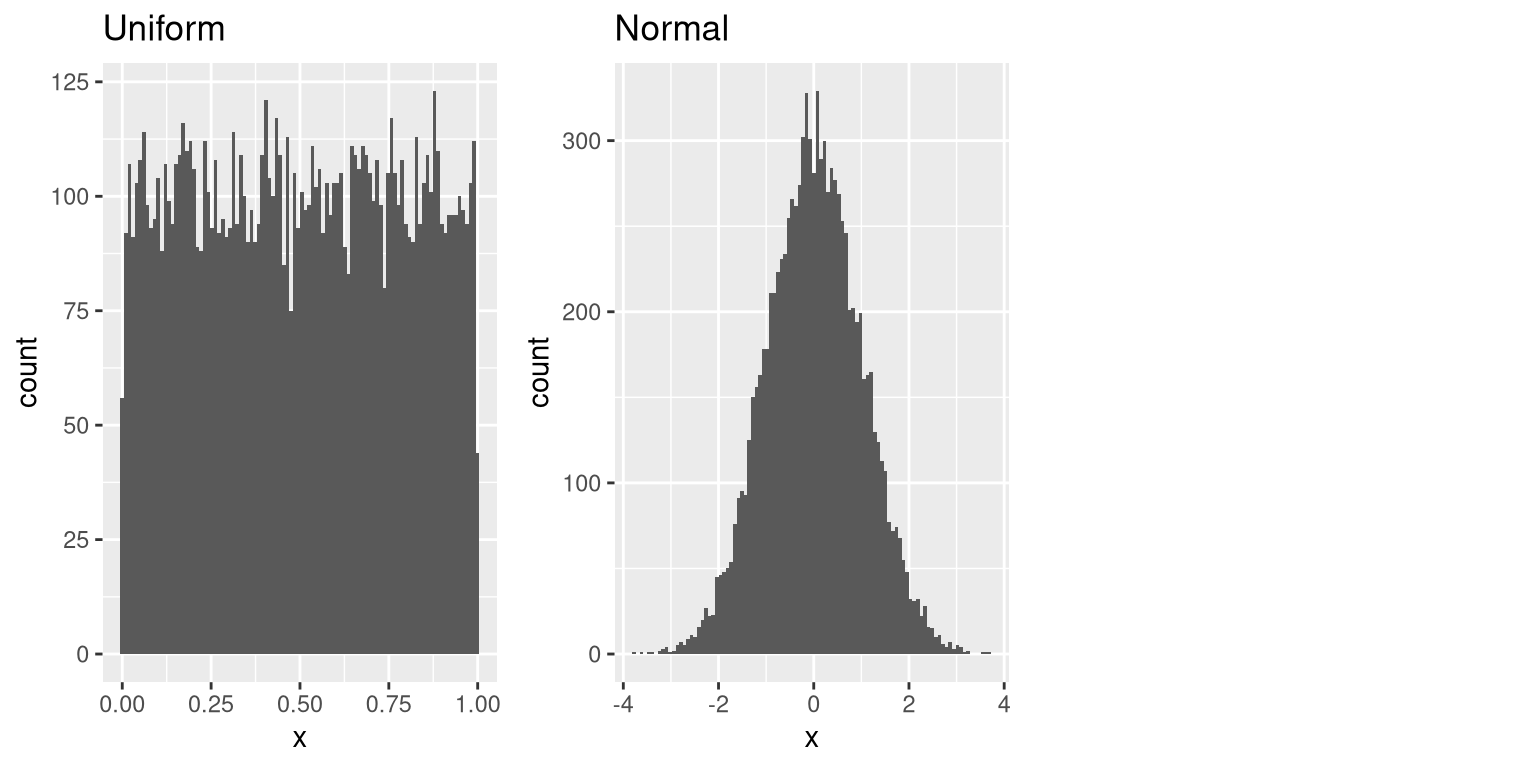
Figure 8.1: Examples of random numbers generated from a uniform (left) or normal (right) distribution.
One can also generate random numbers for any distribution using a quantile function for the distribution. This is the inverse of the cumulative distribution function; instead of identifying the cumulative probabilities for a set of values, the quantile function identifies the values for a set of cumulative probabilities. Using the quantile function, we can generate random numbers from a uniform distribution, and then map those into the distribution of interest via its quantile function.
By default, the random number generators in statistical software will generate a different set of random numbers every time they are run. However, it is also possible to generate exactly the same set of random numbers, by setting what is called the random seed to a specific value. If you were to look at the code that generated these figures, We will do this in many of the examples in this book, in order to make sure that the examples are reproducible.
8.4 Using Monte Carlo simulation
Let’s go back to our example of exam finishing times. Say that I administer three quizzes and record the finishing times for each student for each exam, which might look like the distributions presented in Figure 8.2.
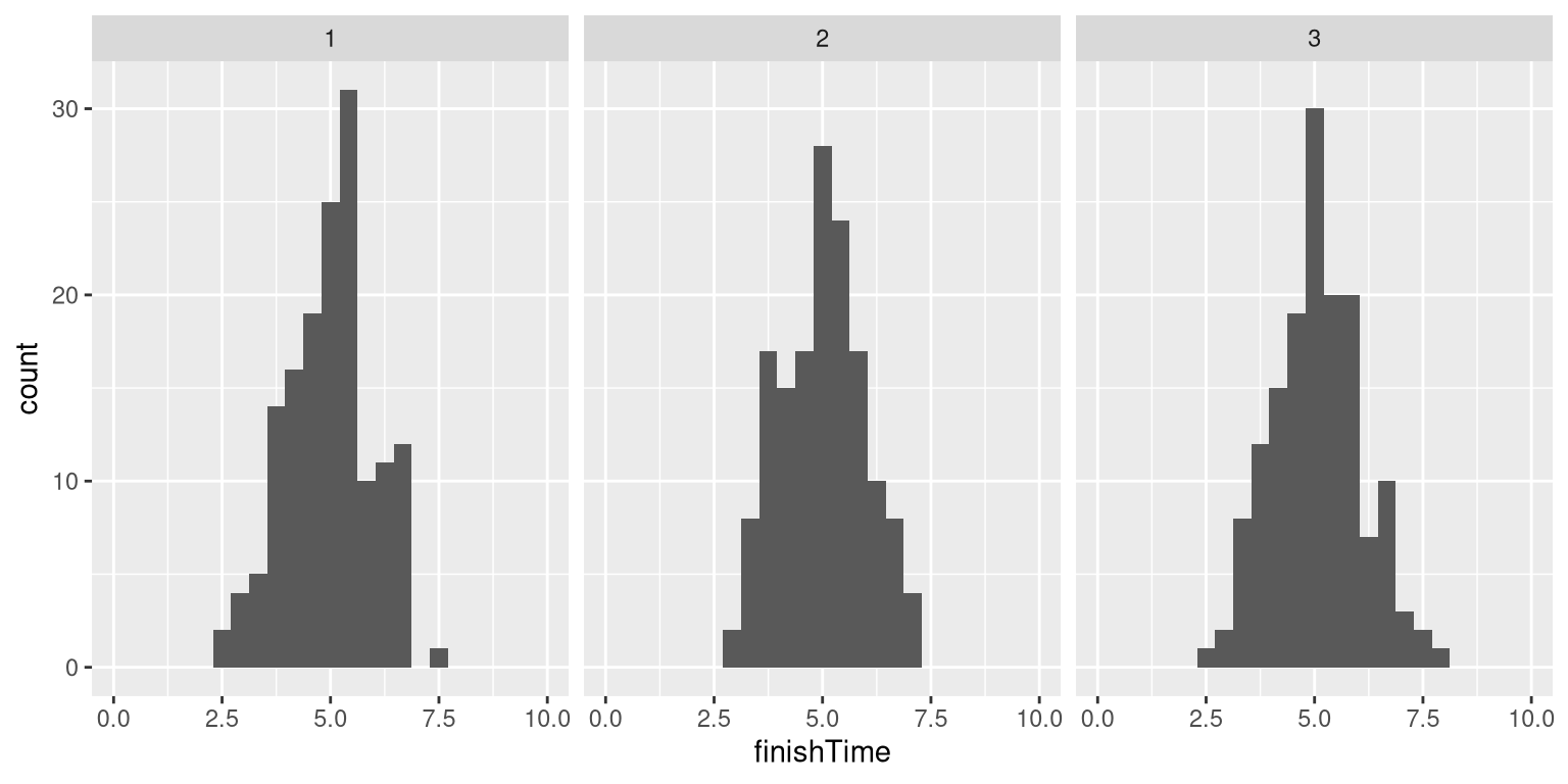
Figure 8.2: Simulated finishing time distributions.
What we really want to know to answer our question is not what the distribution of finishing times looks like, but rather what the distribution of the longest finishing time for each quiz looks like. To do this, we can simulate the finishing time for a quiz, using the assumption that the finishing times are distributed normally, as stated above; for each of these simulated quizzes, we then record the longest finishing time. We repeat this simulation a large number of times (5000 should be enough) and record the distribution of finishing times, which is shown in Figure 8.3.
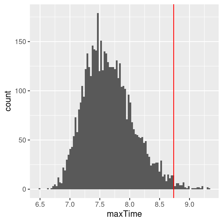
Figure 8.3: Distribution of maximum finishing times across simulations.
This shows that the 99th percentile of the finishing time distribution falls at 8.74, meaning that if we were to give that much time for the quiz, then everyone should finish 99% of the time. It’s always important to remember that our assumptions matter – if they are wrong, then the results of the simulation are useless. In this case, we assumed that the finishing time distribution was normally distributed with a particular mean and standard deviation; if these assumptions are incorrect (and they almost certainly are, since it’s rare for elapsed times to be normally distributed), then the true answer could be very different.
8.5 Using simulation for statistics: The bootstrap
So far we have used simulation to demonstrate statistical principles, but we can also use simulation to answer real statistical questions. In this section we will introduce a concept known as the bootstrap that lets us use simulation to quantify our uncertainty about statistical estimates. Later in the course, we will see other examples of how simulation can often be used to answer statistical questions, especially when theoretical statistical methods are not available or when their assumptions are too difficult to meet.
8.5.1 Computing the bootstrap
In the previous chapter, we used our knowledge of the sampling distribution of the mean to compute the standard error of the mean. But what if we can’t assume that the estimates are normally distributed, or we don’t know their distribution? The idea of the bootstrap is to use the data themselves to estimate an answer. The name comes from the idea of pulling one’s self up by one’s own bootstraps, expressing the idea that we don’t have any external source of leverage so we have to rely upon the data themselves. The bootstrap method was conceived by Bradley Efron of the Stanford Department of Statistics, who is one of the world’s most influential statisticians.
The idea behind the bootstrap is that we repeatedly sample from the actual dataset; importantly, we sample with replacement, such that the same data point will often end up being represented multiple times within one of the samples. We then compute our statistic of interest on each of the bootstrap samples, and use the distribution of those estimates as our sampling distribution. In a sense, we treat our particular sample as the entire population, and then repeatedly sample with replacement to generate our samples for analysis. This makes the assumption that our particular sample is an accurate reflection of the population, which is probably reasonable for larger samples but can break down when samples are smaller.
Let’s start by using the bootstrap to estimate the sampling distribution of the mean of adult height in the NHANES dataset, so that we can compare the result to the standard error of the mean (SEM) that we discussed earlier.
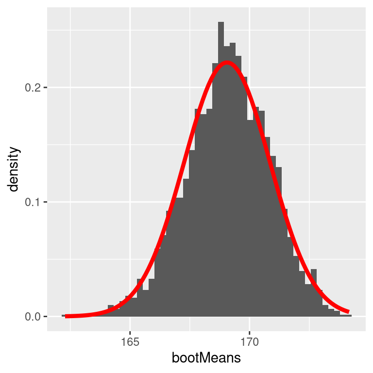
Figure 8.4: An example of bootstrapping to compute the standard error of the mean adult height in the NHANES dataset. The histogram shows the distribution of means across bootstrap samples, while the red line shows the normal distribution based on the sample mean and standard deviation.
Figure 8.4 shows that the distribution of means across bootstrap samples is fairly close to the theoretical estimate based on the assumption of normality. We would not usually employ the bootstrap to compute confidence intervals for the mean (since we can generally assume that the normal distribution is appropriate for the sampling distribution of the mean, as long as our sample is large enough), but this example shows how the method gives us roughly the same result as the standard method based on the normal distribution. The bootstrap would more often be used to generate standard errors for estimates of other statistics where we know or suspect that the normal distribution is not appropriate. In addition, in a later chapter you will see how we can also use the bootstrap samples to generate estimates of the uncertainty in our sample statistic as well.