Chapter 12 Modeling categorical relationships
So far we have discussed the general concepts of statistical modeling and hypothesis testing, and applied them to some simple analyses; now we will turn to the question of how to model particular kinds of relationships in our data. In this chapter we will focus on the modeling of categorical relationships, by which we mean relationships between variables that are measured qualitatively. These data are usually expressed in terms of counts; that is, for each value of the variable (or combination of values of multiple variables), how many observations take that value? For example, when we count how many people from each major are in our class, we are fitting a categorical model to the data.
12.1 Example: Candy colors
Let’s say that I have purchased a bag of 100 candies, which are labeled as having 1/3 chocolates, 1/3 licorices, and 1/3 gumballs. When I count the candies in the bag, we get the following numbers: 30 chocolates, 33 licorices, and 37 gumballs. Because I like chocolate much more than licorice or gumballs, I feel slightly ripped off and I’d like to know if this was just a random accident. To answer that question, I need to know: What is the likelihood that the count would come out this way if the true probability of each candy type is the averaged proportion of 1/3 each?
12.2 Pearson’s chi-squared test
The Pearson chi-squared test provides us with a way to test whether a set of observed counts differs from some specific expected values that define the null hypothesis:
\[ \chi^2 = \sum_i\frac{(observed_i - expected_i)^2}{expected_i} \]
In the case of our candy example, the null hypothesis is that the proportion of each type of candy is equal. To compute the chi-squared statistic, we first need to come up with our expected counts under the null hypothesis: since the null is that they are all the same, then this is just the total count split across the three categories (as shown in Table 12.1). We then take the difference between each count and its expectation under the null hypothesis, square them, divide them by the null expectation, and add them up to obtain the chi-squared statistic.
| Candy Type | count | nullExpectation | squared difference |
|---|---|---|---|
| chocolate | 30 | 33 | 11.11 |
| licorice | 33 | 33 | 0.11 |
| gumball | 37 | 33 | 13.44 |
The chi-squared statistic for this analysis comes out to 0.74, which on its own is not interpretable, since it depends on the number of different values that were added together. However, we can take advantage of the fact that the chi-squared statistic is distributed according to a specific distribution under the null hypothesis, which is known as the chi-squared distribution. This distribution is defined as the sum of squares of a set of standard normal random variables; it has a number of degrees of freedom that is equal to the number of variables being added together. The shape of the distribution depends on the number of degrees of freedom. The left panel of Figure 12.1 shows examples of the distribution for several different degrees of freedom.
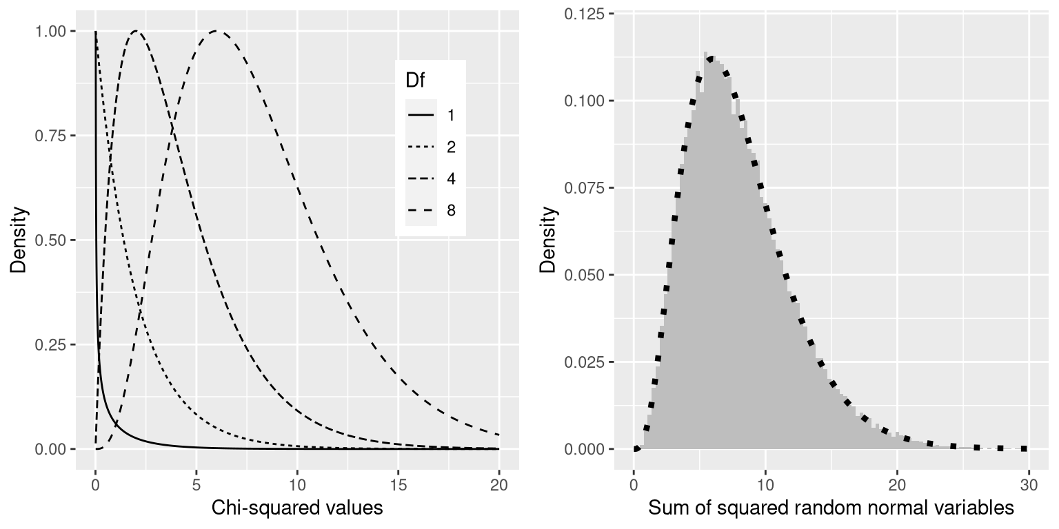
Figure 12.1: Left: Examples of the chi-squared distribution for various degrees of freedom. Right: Simulation of sum of squared random normal variables. The histogram is based on the sum of squares of 50,000 sets of 8 random normal variables; the dotted line shows the values of the theoretical chi-squared distribution with 8 degrees of freedom.
Let’s verify that the chi-squared distribution accurately describes the sum of squares of a set of standard normal random variables, using simulation. To do this, we repeatedly draw sets of 8 random numbers, and add up each set after squaring each value. The right panel of Figure 12.1 shows that the theoretical distribution matches closely with the results of a simulation that repeatedly added together the squares of a set of random normal variables.
For the candy example, we can compute the likelihood of our observed chi-squared value of 0.74 under the null hypothesis of equal frequency across all candies. We use a chi-squared distribution with degrees of freedom equal to k - 1 (where k = the number of categories) since we lost one degree of freedom when we computed the mean in order to generate the expected values. The resulting p-value (P(Chi-squared) > 0.74 = 0.691) shows that the observed counts of candies are not particularly surprising based on the proportions printed on the bag of candy, and we would not reject the null hypothesis of equal proportions.
12.3 Contingency tables and the two-way test
Another way that we often use the chi-squared test is to ask whether two categorical variables are related to one another. As a more realistic example, let’s take the question of whether a Black driver is more likely to be searched when they are pulled over by a police officer, compared to a white driver. The Stanford Open Policing Project (https://openpolicing.stanford.edu/) has studied this, and provides data that we can use to analyze the question. We will use the data from the State of Connecticut since they are fairly small and thus easier to analyze.
The standard way to represent data from a categorical analysis is through a contingency table, which presents the number or proportion of observations falling into each possible combination of values for each of the variables. Table 12.2 below shows the contingency table for the police search data. It can also be useful to look at the contingency table using proportions rather than raw numbers, since they are easier to compare visually, so we include both absolute and relative numbers here.
| searched | Black | White | Black (relative) | White (relative) |
|---|---|---|---|---|
| FALSE | 36244 | 239241 | 0.13 | 0.86 |
| TRUE | 1219 | 3108 | 0.00 | 0.01 |
The Pearson chi-squared test allows us to test whether observed frequencies are different from expected frequencies, so we need to determine what frequencies we would expect in each cell if searches and race were unrelated – which we can define as being independent. Remember from the chapter on probability that if X and Y are independent, then:
\[ P(X \cap Y) = P(X) * P(Y) \] That is, the joint probability under the null hypothesis of independence is simply the product of the marginal probabilities of each individual variable. The marginal probabilities are simply the probabilities of each event occuring regardless of other events. We can compute those marginal probabilities, and then multiply them together to get the expected proportions under independence.
| Black | White | ||
|---|---|---|---|
| Not searched | P(NS)*P(B) | P(NS)*P(W) | P(NS) |
| Searched | P(S)*P(B) | P(S)*P(W) | P(S) |
| P(B) | P(W) |
We then compute the chi-squared statistic, which comes out to 828.3. To compute a p-value, we need to compare it to the null chi-squared distribution in order to determine how extreme our chi-squared value is compared to our expectation under the null hypothesis. The degrees of freedom for this distribution are \(df = (nRows - 1) * (nColumns - 1)\) - thus, for a 2X2 table like the one here, \(df = (2-1)*(2-1)=1\). The intuition here is that computing the expected frequencies requires us to use three values: the total number of observations and the marginal probability for each of the two variables. Thus, once those values are computed, there is only one number that is free to vary, and thus there is one degree of freedom. Given this, we can compute the p-value for the chi-squared statistic, which is about as close to zero as one can get: \(3.79 \times 10^{-182}\). This shows that the observed data would be highly unlikely if there was truly no relationship between race and police searches, and thus we should reject the null hypothesis of independence.
We can also perform this test easily using our statistical software:
##
##  Pearson's Chi-squared test
##
## data:  summaryDf2wayTable and 1
## X-squared = 828, df = 1, p-value <2e-16
12.4 Standardized residuals
When we find a significant effect with the chi-squared test, this tells us that the data are unlikely under the null hypothesis, but it doesn’t tell us how the data differ. To get a deeper insight into how the data differ from what we would expect under the null hypothesis, we can examine the residuals from the model, which reflects the deviation of the data (i.e., the observed frequencies) from the model (i.e., the expected frequencies) in each cell. Rather than looking at the raw residuals (which will vary simply depending on the number of observations in the data), it’s more common to look at the standardized residuals (sometimes called Pearson residuals), which are computed as:
\[ standardized\ residual_{ij} = \frac{observed_{ij} - expected_{ij}}{\sqrt{expected_{ij}}} \] where \(i\) and \(j\) are the indices for the rows and columns respectively.
Table 12.3 shows these for the police stop data. These standardized residuals can be interpreted as Z scores – in this case, we see that the number of searches for Black individuals are substantially higher than expected based on independence, and the number of searches for white individuals are substantially lower than expected. This provides us with the context that we need to interpret the signficant chi-squared result.
| searched | driver_race | Standardized residuals |
|---|---|---|
| FALSE | Black | -3.3 |
| TRUE | Black | 26.6 |
| FALSE | White | 1.3 |
| TRUE | White | -10.4 |
12.5 Odds ratios
We can also represent the relative likelihood of different outcomes in the contingency table using the odds ratio that we introduced earlier, in order to better understand the magnitude of the effect. First, we represent the odds of being stopped for each race, then we compute their ratio:
\[ odds_{searched|black} = \frac{N_{searched\cap black}}{N_{not\ searched\cap black}} = \frac{1219}{36244} = 0.034 \]
\[ odds_{searched|white} = \frac{N_{searched\cap white}}{N_{not\ searched\cap white}} = \frac{3108}{239241} = 0.013 \] \[ odds\ ratio = \frac{odds_{searched|black}}{odds_{searched|white}} = 2.59 \]
The odds ratio shows that the odds of being searched are 2.59 times higher for Black versus white drivers, based on this dataset.
12.6 Bayes factor
We discussed Bayes factors in the earlier chapter on Bayesian statistics – you may remember that it represents the ratio of the likelihood of the data under each of the two hypotheses: \[ K = \frac{P(data|H_A)}{P(data|H_0)} = \frac{P(H_A|data)*P(H_A)}{P(H_0|data)*P(H_0)} \] We can compute the Bayes factor for the police search data using our statistical software:
## Bayes factor analysis
## --------------
## [1] Non-indep. (a=1) : 1.8e+142 ±0%
##
## Against denominator:
##   Null, independence, a = 1
## ---
## Bayes factor type: BFcontingencyTable, independent multinomial
This shows that the evidence in favor of a relationship between driver race and police searches in this dataset is exceedingly strong — \(1.8 * 10^{142}\) is about as close to infinity as we can imagine getting in statistics.
12.7 Categorical analysis beyond the 2 X 2 table
Categorical analysis can also be applied to contingency tables where there are more than two categories for each variable.
For example, let’s look at the NHANES data and compare the variable Depressed which denotes the “self-reported number of days where the participant felt down, depressed or hopeless”. This variable is coded as None, Several, or Most. Let’s test whether this variable is related to the SleepTrouble variable which denotes whether the individual has reported sleeping problems to a doctor.
| Depressed | NoSleepTrouble | YesSleepTrouble |
|---|---|---|
| None | 2614 | 676 |
| Several | 418 | 249 |
| Most | 138 | 145 |
Simply by looking at these data, we can tell that it is likely that there is a relationship between the two variables; notably, while the total number of people with sleep trouble is much less than those without, for people who report being depresssed most days the number with sleep problems is greater than those without. We can quantify this directly using the chi-squared test:
##
##  Pearson's Chi-squared test
##
## data:  depressedSleepTroubleTable
## X-squared = 191, df = 2, p-value <2e-16
This test shows that there is a strong relationship between depression and sleep trouble. We can also compute the Bayes factor to quantify the strength of the evidence in favor of the alternative hypothesis:
## Bayes factor analysis
## --------------
## [1] Non-indep. (a=1) : 1.8e+35 ±0%
##
## Against denominator:
##   Null, independence, a = 1
## ---
## Bayes factor type: BFcontingencyTable, joint multinomial
Here we see that the Bayes factor is very large (\(1.8 * 10^{35}\)), showing that the evidence in favor of a relation between depression and sleep problems is very strong.
12.8 Beware of Simpson’s paradox
The contingency tables presented above represent summaries of large numbers of observations, but summaries can sometimes be misleading. Let’s take an example from baseball. The table below shows the batting data (hits/at bats and batting average) for Derek Jeter and David Justice over the years 1995-1997:
| Player | 1995 | 1996 | 1997 | Combined | ||||
|---|---|---|---|---|---|---|---|---|
| Derek Jeter | 12/48 | .250 | 183/582 | .314 | 190/654 | .291 | 385/1284 | .300 |
| David Justice | 104/411 | .253 | 45/140 | .321 | 163/495 | .329 | 312/1046 | .298 |
If you look closely, you will see that something odd is going on: In each individual year Justice had a higher batting average than Jeter, but when we combine the data across all three years, Jeter’s average is actually higher than Justice’s! This is an example of a phenomenon known as Simpson’s paradox, in which a pattern that is present in a combined dataset may not be present in any of the subsets of the data. This occurs when there is another variable that may be changing across the different subsets – in this case, the number of at-bats varies across years, with Justice batting many more times in 1995 (when batting averages were low). We refer to this as a lurking variable, and it’s always important to be attentive to such variables whenever one examines categorical data.
12.9 Learning objectives
- Describe the concept of a contingency table for categorical data.
- Describe the concept of the chi-squared test for association and compute it for a given contingency table.
- Describe Simpson’s paradox and why it is important for categorical data analysis.