Chapter 2 Working with data
2.1 What are data?
The first important point about data is that data are – meaning that the word “data” is plural (though some people disagree with me on this). You might also wonder how to pronounce “data” – I say “day-tah”, but I know many people who say “dah-tah”, and I have been able to remain friends with them in spite of this. Now, if I heard them say “the data is” then that would be a bigger issue…
2.1.1 Qualitative data
Data are composed of variables, where a variable reflects a unique measurement or quantity. Some variables are qualitative, meaning that they describe a quality rather than a numeric quantity. For example, in my stats course I generally give an introductory survey, both to obtain data to use in class and to learn more about the students. One of the questions that I ask is “What is your favorite food?”, to which some of the answers have been: blueberries, chocolate, tamales, pasta, pizza, and mango. Those data are not intrinsically numerical; we could assign numbers to each one (1=blueberries, 2=chocolate, etc), but we would just be using the numbers as labels rather than as real numbers. This also constrains what we should do with those numbers; for example, it wouldn’t make sense to compute the average of those numbers. However, we will often code qualitative data using numbers in order to make them easier to work with, as you will see later.
2.1.2 Quantitative data
More commonly in statistics we will work with quantitative data, meaning data that are numerical. For example, here Table 2.1 shows the results from another question that I ask in my introductory class, which is “Why are you taking this class?”
| Why are you taking this class? | Number of students |
|---|---|
| It fulfills a degree plan requirement | 105 |
| It fulfills a General Education Breadth Requirement | 32 |
| It is not required but I am interested in the topic | 11 |
| Other | 4 |
Note that the students’ answers were qualitative, but we generated a quantitative summary of them by counting how many students gave each response.
2.1.2.1 Types of numbers
There are several different types of numbers that we work with in statistics. It’s important to understand these differences, in part because statistical analysis languages (such as R) often distinguish between them.
Binary numbers. The simplest are binary numbers – that is, zero or one. We will often use binary numbers to represent whether something is true or false, or present or absent. For example, I might ask 10 people if they have ever experienced a migraine headache, recording their answers as “Yes” or “No”. It’s often useful to instead use logical values, which take the value of either TRUE or FALSE. This can be especially useful when we start using programming languages like R to analyze our data, since these languages already understand the concepts of TRUE and FALSE. In fact, most programming languages treat truth values and binary numbers equivalently. The number 1 is equal to the logical value TRUE, and the number zero is equal to the logical value FALSE.
Integers. Integers are whole numbers with no fractional or decimal part. We most commonly encounter integers when we count things, but they also often occur in psychological measurement. For example, in my introductory survey I administer a set of questions about attitudes towards statistics (such as “Statistics seems very mysterious to me.”), on which the students respond with a number between 1 (“Disagree strongly”) and 7 (“Agree strongly”).
Real numbers. Most commonly in statistics we work with real numbers, which have a fractional/decimal part. For example, we might measure someone’s weight, which can be measured to an arbitrary level of precision, from kilograms down to micrograms.
2.2 Discrete versus continuous measurements
A discrete measurement is one that takes one of a finite set of particular values. These could be qualitative values (for example, different breeds of dogs) or numerical values (for example, how many friends one has on Facebook). Importantly, there is no middle ground between the measurements; it doesn’t make sense to say that one has 33.7 friends.
A continuous measurement is one that is defined in terms of a real number. It could fall anywhere in a particular range of values, though usually our measurement tools will limit the precision with which we can measure it; for example, a floor scale might measure weight to the nearest kg, even though weight could in theory be measured with much more precision.
It is common in statistics courses to go into more detail about different “scales” of measurement, which are discussed in more detail in the Appendix to this chapter. The most important takeaway from this is that some kinds of statistics don’t make sense on some kinds of data. For example, imagine that we were to collect postal Zip Code data from a number of individuals. Those numbers are represented as integers, but they don’t actually refer to a numeric scale; each zip code basically serves as a label for a different region. For this reason, it wouldn’t make sense to talk about the average zip code, for example.
2.3 What makes a good measurement?
In many fields such as psychology, the thing that we are measuring is not a physical feature, but instead is an unobservable theoretical concept, which we usually refer to as a construct. For example, let’s say that I want to test how well you understand the distinction between the different types of numbers described above. I could give you a pop quiz that would ask you several questions about these concepts and count how many you got right. This test might or might not be a good measurement of the construct of your actual knowledge – for example, if I were to write the test in a confusing way or use language that you don’t understand, then the test might suggest you don’t understand the concepts when really you do. On the other hand, if I give a multiple choice test with very obvious wrong answers, then you might be able to perform well on the test even if you don’t actually understand the material.
It is usually impossible to measure a construct without some amount of error. In the example above, you might know the answer, but you might mis-read the question and get it wrong. In other cases, there is error intrinsic to the thing being measured, such as when we measure how long it takes a person to respond on a simple reaction time test, which will vary from trial to trial for many reasons. We generally want our measurement error to be as low as possible, which we can achieve either by improving the quality of the measurement (for example, using a better time to measure reaction time), or by averaging over a larger number of indvidiual measurements.
Sometimes there is a standard against which other measurements can be tested, which we might refer to as a “gold standard” – for example, measurement of sleep can be done using many different devices (such as devices that measure movement in bed), but they are generally considered inferior to the gold standard of polysomnography (which uses measurement of brain waves to quantify the amount of time a person spends in each stage of sleep). Often the gold standard is more difficult or expensive to perform, and the cheaper method is used even though it might have greater error.
When we think about what makes a good measurement, we usually distinguish two different aspects of a good measurement: it should be reliable, and it should be valid.
2.3.1 Reliability
Reliability refers to the consistency of our measurements. One common form of reliability, known as “test-retest reliability”, measures how well the measurements agree if the same measurement is performed twice. For example, I might give you a questionnaire about your attitude towards statistics today, repeat this same questionnaire tomorrow, and compare your answers on the two days; we would hope that they would be very similar to one another, unless something happened in between the two tests that should have changed your view of statistics (like reading this book!).
Another way to assess reliability comes in cases where the data include subjective judgments. For example, let’s say that a researcher wants to determine whether a treatment changes how well an autistic child interacts with other children, which is measured by having experts watch the child and rate their interactions with the other children. In this case we would like to make sure that the answers don’t depend on the individual rater — that is, we would like for there to be high inter-rater reliability. This can be assessed by having more than one rater perform the rating, and then comparing their ratings to make sure that they agree well with one another.
Reliability is important if we want to compare one measurement to another, because the relationship between two different variables can’t be any stronger than the relationship between either of the variables and itself (i.e., its reliability). This means that an unreliable measure can never have a strong statistical relationship with any other measure. For this reason, researchers developing a new measurement (such as a new survey) will often go to great lengths to establish and improve its reliability.
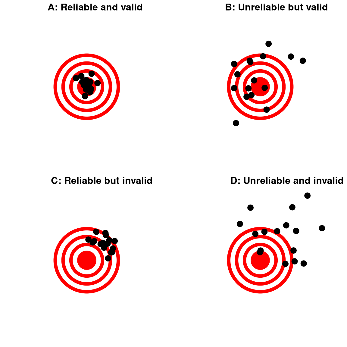
Figure 2.1: A figure demonstrating the distinction between reliability and validity, using shots at a bullseye. Reliability refers to the consistency of location of shots, and validity refers to the accuracy of the shots with respect to the center of the bullseye.
2.3.2 Validity
Reliability is important, but on its own it’s not enough: After all, I could create a perfectly reliable measurement on a personality test by re-coding every answer using the same number, regardless of how the person actually answers. We want our measurements to also be valid — that is, we want to make sure that we are actually measuring the construct that we think we are measuring (Figure 2.1). There are many different types of validity that are commonly discussed; we will focus on three of them.
Face validity. Does the measurement make sense on its face? If I were to tell you that I was going to measure a person’s blood pressure by looking at the color of their tongue, you would probably think that this was not a valid measure on its face. On the other hand, using a blood pressure cuff would have face validity. This is usually a first reality check before we dive into more complicated aspects of validity.
Construct validity. Is the measurement related to other measurements in an appropriate way? This is often subdivided into two aspects. Convergent validity means that the measurement should be closely related to other measures that are thought to reflect the same construct. Let’s say that I am interested in measuring how extroverted a person is using either a questionnaire or an interview. Convergent validity would be demonstrated if both of these different measurements are closely related to one another. On the other hand, measurements thought to reflect different constructs should be unrelated, known as divergent validity. If my theory of personality says that extraversion and conscientiousness are two distinct constructs, then I should also see that my measurements of extraversion are unrelated to measurements of conscientiousness.
Predictive validity. If our measurements are truly valid, then they should also be predictive of other outcomes. For example, let’s say that we think that the psychological trait of sensation seeking (the desire for new experiences) is related to risk taking in the real world. To test for predictive validity of a measurement of sensation seeking, we would test how well scores on the test predict scores on a different survey that measures real-world risk taking.
2.4 Learning Objectives
Having read this chapter, you should be able to:
- Distinguish between different types of variables (quantitative/qualitative, binary/integer/real, discrete/continuous) and give examples of each of these kinds of variables
- Distinguish between the concepts of reliability and validity and apply each concept to a particular dataset
2.5 Suggested readings
- An Introduction to Psychometric Theory with Applications in R - A free online textbook on psychological measurement
2.6 Appendix
2.6.1 Scales of measurement
All variables must take on at least two different possible values (otherwise they would be a constant rather than a variable), but different values of the variable can relate to each other in different ways, which we refer to as scales of measurement. There are four ways in which the different values of a variable can differ.
- Identity: Each value of the variable has a unique meaning.
- Magnitude: The values of the variable reflect different magnitudes and have an ordered relationship to one another – that is, some values are larger and some are smaller.
- Equal intervals: Units along the scale of measurement are equal to one another. This means, for example, that the difference between 1 and 2 would be equal in its magnitude to the difference between 19 and 20.
- Absolute zero: The scale has a true meaningful zero point. For example, for many measurements of physical quantities such as height or weight, this is the complete absence of the thing being measured.
There are four different scales of measurement that go along with these different ways that values of a variable can differ.
Nominal scale. A nominal variable satisfies the criterion of identity, such that each value of the variable represents something different, but the numbers simply serve as qualitative labels as discussed above. For example, we might ask people for their political party affiliation, and then code those as numbers: 1 = “Republican”, 2 = “Democrat”, 3 = “Libertarian”, and so on. However, the different numbers do not have any ordered relationship with one another.
Ordinal scale. An ordinal variable satisfies the criteria of identity and magnitude, such that the values can be ordered in terms of their magnitude. For example, we might ask a person with chronic pain to complete a form every day assessing how bad their pain is, using a 1-7 numeric scale. Note that while the person is presumably feeling more pain on a day when they report a 6 versus a day when they report a 3, it wouldn’t make sense to say that their pain is twice as bad on the former versus the latter day; the ordering gives us information about relative magnitude, but the differences between values are not necessarily equal in magnitude.
Interval scale. An interval scale has all of the features of an ordinal scale, but in addition the intervals between units on the measurement scale can be treated as equal. A standard example is physical temperature measured in Celsius or Fahrenheit; the physical difference between 10 and 20 degrees is the same as the physical difference between 90 and 100 degrees, but each scale can also take on negative values.
Ratio scale. A ratio scale variable has all four of the features outlined above: identity, magnitude, equal intervals, and absolute zero. The difference between a ratio scale variable and an interval scale variable is that the ratio scale variable has a true zero point. Examples of ratio scale variables include physical height and weight, along with temperature measured in Kelvin.
There are two important reasons that we must pay attention to the scale of measurement of a variable. First, the scale determines what kind of mathematical operations we can apply to the data (see Table 2.2). A nominal variable can only be compared for equality; that is, do two observations on that variable have the same numeric value? It would not make sense to apply other mathematical operations to a nominal variable, since they don’t really function as numbers in a nominal variable, but rather as labels. With ordinal variables, we can also test whether one value is greater or lesser than another, but we can’t do any arithmetic. Interval and ratio variables allow us to perform arithmetic; with interval variables we can only add or subtract values, whereas with ratio variables we can also multiply and divide values.
| Equal/not equal | >/< | +/- | Multiply/divide | |
|---|---|---|---|---|
| Nominal | OK | |||
| Ordinal | OK | OK | ||
| Interval | OK | OK | OK | |
| Ratio | OK | OK | OK | OK |
These constraints also imply that there are certain kinds of statistics that we can compute on each type of variable. Statistics that simply involve counting of different values (such as the most common value, known as the mode), can be calculated on any of the variable types. Other statistics are based on ordering or ranking of values (such as the median, which is the middle value when all of the values are ordered by their magnitude), and these require that the value at least be on an ordinal scale. Finally, statistics that involve adding up values (such as the average, or mean), require that the variables be at least on an interval scale. Having said that, we should note that it’s quite common for researchers to compute the mean of variables that are only ordinal (such as responses on personality tests), but this can sometimes be problematic.