Chapter 9 Hypothesis testing

In the first chapter we discussed the three major goals of statistics:

• Describe
• Decide
• Predict

In this chapter we will introduce the ideas behind the use of statistics to make decisions – in particular, decisions about whether a particular hypothesis is supported by the data.

9.1 Null Hypothesis Statistical Testing (NHST)

The specific type of hypothesis testing that we will discuss is known (for reasons that will become clear) as null hypothesis statistical testing (NHST). If you pick up almost any scientific or biomedical research publication, you will see NHST being used to test hypotheses, and in their introductory psychology textbook, Gerrig & Zimbardo (2002) referred to NHST as the “backbone of psychological research”. Thus, learning how to use and interpret the results from hypothesis testing is essential to understand the results from many fields of research.

It is also important for you to know, however, that NHST is deeply flawed, and that many statisticians and researchers (including myself) think that it has been the cause of serious problems in science, which we will discuss in Chapter 18. For more than 50 years, there have been calls to abandon NHST in favor of other approaches (like those that we will discuss in the following chapters):

• “The test of statistical significance in psychological research may be taken as an instance of a kind of essential mindlessness in the conduct of research” (Bakan, 1966)
• Hypothesis testing is “a wrongheaded view about what constitutes scientific progress” (Luce, 1988)

NHST is also widely misunderstood, largely because it violates our intuitions about how statistical hypothesis testing should work. Let’s look at an example to see this.

9.2 Null hypothesis statistical testing: An example

There is great interest in the use of body-worn cameras by police officers, which are thought to reduce the use of force and improve officer behavior. However, in order to establish this we need experimental evidence, and it has become increasingly common for governments to use randomized controlled trials to test such ideas. A randomized controlled trial of the effectiveness of body-worn cameras was performed by the Washington, DC government and DC Metropolitan Police Department in 2015/2016. Officers were randomly assigned to wear a body-worn camera or not, and their behavior was then tracked over time to determine whether the cameras resulted in less use of force and fewer civilian complaints about officer behavior.

Before we get to the results, let’s ask how you would think the statistical analysis might work. Let’s say we want to specifically test the hypothesis of whether the use of force is decreased by the wearing of cameras. The randomized controlled trial provides us with the data to test the hypothesis – namely, the rates of use of force by officers assigned to either the camera or control groups. The next obvious step is to look at the data and determine whether they provide convincing evidence for or against this hypothesis. That is: What is the likelihood that body-worn cameras reduce the use of force, given the data and everything else we know?

It turns out that this is not how null hypothesis testing works. Instead, we first take our hypothesis of interest (i.e. that body-worn cameras reduce use of force), and flip it on its head, creating a null hypothesis – in this case, the null hypothesis would be that cameras do not reduce use of force. Importantly, we then assume that the null hypothesis is true. We then look at the data, and determine how likely the data would be if the null hypothesis were true. If the the data are sufficiently unlikely under the null hypothesis that we can reject the null in favor of the alternative hypothesis which is our hypothesis of interest. If there is not sufficient evidence to reject the null, then we say that we retain (or “fail to reject”) the null, sticking with our initial assumption that the null is true.

Understanding some of the concepts of NHST, particularly the notorious “p-value”, is invariably challenging the first time one encounters them, because they are so counter-intuitive. As we will see later, there are other approaches that provide a much more intuitive way to address hypothesis testing (but have their own complexities). However, before we get to those, it’s important for you to have a deep understanding of how hypothesis testing works, because it’s clearly not going to go away any time soon.

9.3 The process of null hypothesis testing

We can break the process of null hypothesis testing down into a number of steps:

1. Formulate a hypothesis that embodies our prediction (before seeing the data)
2. Specify null and alternative hypotheses
3. Collect some data relevant to the hypothesis
4. Fit a model to the data that represents the alternative hypothesis and compute a test statistic
5. Compute the probability of the observed value of that statistic assuming that the null hypothesis is true
6. Assess the “statistical significance” of the result

For a hands-on example, let’s use the NHANES data to ask the following question: Is physical activity related to body mass index? In the NHANES dataset, participants were asked whether they engage regularly in moderate or vigorous-intensity sports, fitness or recreational activities (stored in the variable \(PhysActive\)). The researchers also measured height and weight and used them to compute the Body Mass Index (BMI):

\[ BMI = \frac{weight(kg)}{height(m)^2} \]

9.3.1 Step 1: Formulate a hypothesis of interest

We hypothesize that BMI is greater for people who do not engage in physical activity, compared to those who do.

9.3.2 Step 2: Specify the null and alternative hypotheses

For step 2, we need to specify our null hypothesis (which we call \(H_0\)) and our alternative hypothesis (which we call \(H_A\)). \(H_0\) is the baseline against which we test our hypothesis of interest: that is, what would we expect the data to look like if there was no effect? The null hypothesis always involves some kind of equality (=, \(\le\), or \(\ge\)). \(H_A\) describes what we expect if there actually is an effect. The alternative hypothesis always involves some kind of inequality (\(\ne\), >, or <). Importantly, null hypothesis testing operates under the assumption that the null hypothesis is true unless the evidence shows otherwise.

We also have to decide whether we want to test a directional or non-directional hypotheses. A non-directional hypothesis simply predicts that there will be a difference, without predicting which direction it will go. For the BMI/activity example, a non-directional null hypothesis would be:

\(H0: BMI_{active} = BMI_{inactive}\)

and the corresponding non-directional alternative hypothesis would be:

\(HA: BMI_{active} \neq BMI_{inactive}\)

A directional hypothesis, on the other hand, predicts which direction the difference would go. For example, we have strong prior knowledge to predict that people who engage in physical activity should weigh less than those who do not, so we would propose the following directional null hypothesis:

\(H0: BMI_{active} \ge BMI_{inactive}\)

and directional alternative:

\(HA: BMI_{active} < BMI_{inactive}\)

As we will see later, testing a non-directional hypothesis is more conservative, so this is generally to be preferred unless there is a strong a priori reason to hypothesize an effect in a particular direction. Hypotheses, including whether they are directional or not, should always be specified prior to looking at the data!

9.3.3 Step 3: Collect some data

In this case, we will sample 250 individuals from the NHANES dataset. Figure 9.1 shows an example of such a sample, with BMI shown separately for active and inactive individuals, and Table 9.1 shows summary statistics for each group.

Table 9.1: Summary of BMI data for active versus inactive individuals

PhysActive	N	mean	sd
No	131	30	9.0
Yes	119	27	5.2

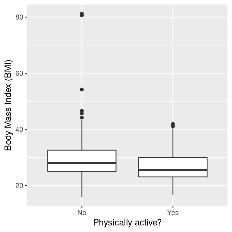
Figure 9.1: Box plot of BMI data from a sample of adults from the NHANES dataset, split by whether they reported engaging in regular physical activity.

9.3.4 Step 4: Fit a model to the data and compute a test statistic

We next want to use the data to compute a statistic that will ultimately let us decide whether the null hypothesis is rejected or not. To do this, the model needs to quantify the amount of evidence in favor of the alternative hypothesis, relative to the variability in the data. Thus we can think of the test statistic as providing a measure of the size of the effect compared to the variability in the data. In general, this test statistic will have a probability distribution associated with it, because that allows us to determine how likely our observed value of the statistic is under the null hypothesis.

For the BMI example, we need a test statistic that allows us to test for a difference between two means, since the hypotheses are stated in terms of mean BMI for each group. One statistic that is often used to compare two means is the t statistic, first developed by the statistician William Sealy Gossett, who worked for the Guiness Brewery in Dublin and wrote under the pen name “Student” - hence, it is often called “Student’s t statistic”. The t statistic is appropriate for comparing the means of two groups when the sample sizes are relatively small and the population standard deviation is unknown. The t statistic for comparison of two independent groups is computed as:

\[ t = \frac{\bar{X_1} - \bar{X_2}}{\sqrt{\frac{S_1^2}{n_1} + \frac{S_2^2}{n_2}}} \]

where \(\bar{X}_1\) and \(\bar{X}_2\) are the means of the two groups, \(S^2_1\) and \(S^2_2\) are the estimated variances of the groups, and \(n_1\) and \(n_2\) are the sizes of the two groups. Because the variance of a difference between two independent variables is the sum of the variances of each individual variable (\(var(A - B) = var(A) + var(B)\)), we add the variances for each group divided by their sample sizes in order to compute the standard error of the difference. Thus, one can view the the t statistic as a way of quantifying how large the difference between groups is in relation to the sampling variability of the difference between means.

The t statistic is distributed according to a probability distribution known as a t distribution. The t distribution looks quite similar to a normal distribution, but it differs depending on the number of degrees of freedom. When the degrees of freedom are large (say 1000), then the t distribution looks essentially like the normal distribution, but when they are small then the t distribution has longer tails than the normal (see Figure 9.2). In the simplest case, where the groups are the same size and have equal variance, the degrees of freedom for the t test is the number of observations minus 2, since we have computed two means and thus given up two degrees of freedom. In this case it’s pretty clear from the box plot that the inactive group is more variable than then active group, and the numbers in each group differ, so we need to use a slightly more complex formula for the degrees of freedom, which is often referred to as a “Welch t-test”. The formula is:

\[ \mathrm{d.f.} = \frac{\left(\frac{S_1^2}{n_1} + \frac{S_2^2}{n_2}\right)^2}{\frac{\left(S_1^2/n_1\right)^2}{n_1-1} + \frac{\left(S_2^2/n_2\right)^2}{n_2-1}} \] This will be equal to \(n_1 + n_2 - 2\) when the variances and sample sizes are equal, and otherwise will be smaller, in effect imposing a penalty on the test for differences in sample size or variance. For this example, that comes out to 241.12 which is slightly below the value of 248 that one would get by subtracting 2 from the sample size.

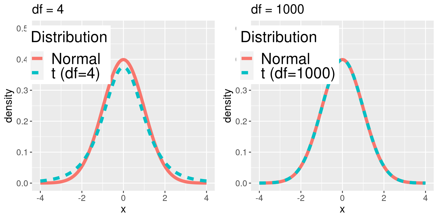
Figure 9.2: Each panel shows the t distribution (in blue dashed line) overlaid on the normal distribution (in solid red line). The left panel shows a t distribution with 4 degrees of freedom, in which case the distribution is similar but has slightly wider tails. The right panel shows a t distribution with 1000 degrees of freedom, in which case it is virtually identical to the normal.

9.3.5 Step 5: Determine the probability of the observed result under the null hypothesis

This is the step where NHST starts to violate our intuition. Rather than determining the likelihood that the null hypothesis is true given the data, we instead determine the likelihood under the null hypothesis of observing a statistic at least as extreme as one that we have observed — because we started out by assuming that the null hypothesis is true! To do this, we need to know the expected probability distribution for the statistic under the null hypothesis, so that we can ask how likely the result would be under that distribution. Note that when I say “how likely the result would be”, what I really mean is “how likely the observed result or one more extreme would be”. There are (at least) two reasons that we need to add this caveat. The first is that when we are talking about continuous values, the probability of any particular value is zero (as you might remember if you’ve taken a calculus class). More importantly, we are trying to determine how weird our result would be if the null hypothesis were true, and any result that is more extreme will be even more weird, so we want to count all of those weirder possibilities when we compute the probability of our result under the null hypothesis.

We can obtain this “null distribution” either using a theoretical distribution (like the t distribution), or using randomization. Before we move to our BMI example, let’s start with some simpler examples.

9.3.5.1 P-values: A very simple example

Let’s say that we wish to determine whether a particular coin is biased towards landing heads. To collect data, we flip the coin 100 times, and let’s say we count 70 heads. In this example, \(H_0: P(heads) \le 0.5\) and \(H_A: P(heads) > 0.5\), and our test statistic is simply the number of heads that we counted. The question that we then want to ask is: How likely is it that we would observe 70 or more heads in 100 coin flips if the true probability of heads is 0.5? We can imagine that this might happen very occasionally just by chance, but doesn’t seem very likely. To quantify this probability, we can use the binomial distribution:

\[ P(X \le k) = \sum_{i=0}^k \binom{N}{k} p^i (1-p)^{(n-i)} \] This equation will tell us the probability of a certain number of heads (\(k\)) or fewer, given a particular probability of heads (\(p\)) and number of events (\(N\)). However, what we really want to know is the probability of a certain number or more, which we can obtain by subtracting from one, based on the rules of probability:

\[ P(X \ge k) = 1 - P(X < k) \]

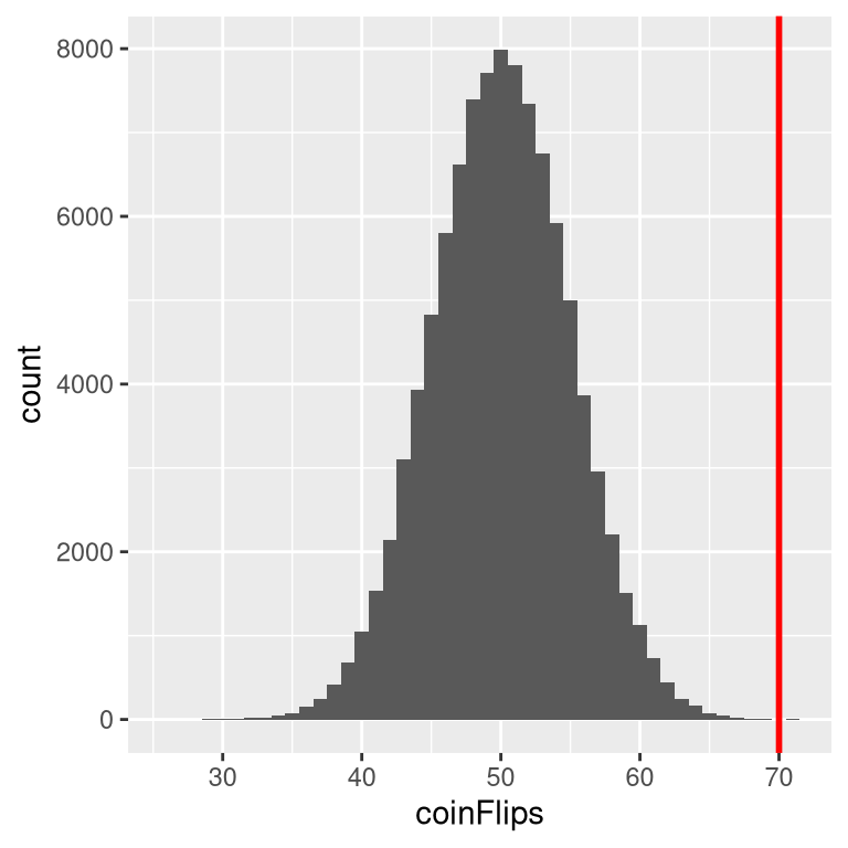
Figure 9.3: Distribution of numbers of heads (out of 100 flips) across 100,000 simulated runs with the observed value of 70 flips represented by the vertical line.

Using the binomial distribution, the probability of 69 or fewer heads given P(heads)=0.5 is 0.999961, so the probability of 70 or more heads is simply one minus that value (0.000039). This computation shows us that the likelihood of getting 70 or more heads if the coin is indeed fair is very small.

Now, what if we didn’t have a standard function to tell us the probability of that number of heads? We could instead determine it by simulation – we repeatedly flip a coin 100 times using a true probability of 0.5, and then compute the distribution of the number of heads across those simulation runs. Figure 9.3 shows the result from this simulation. Here we can see that the probability computed via simulation (0.000030) is very close to the theoretical probability (0.000039).

9.3.5.2 Computing p-values using the t distribution

Now let’s compute a p-value for our BMI example using the t distribution. First we compute the t statistic using the values from our sample that we calculated above, where we find that t = 3.86. The question that we then want to ask is: What is the likelihood that we would find a t statistic of this size, if the true difference between groups is zero or less (i.e. the directional null hypothesis)?

We can use the t distribution to determine this probability. Above we noted that the appropriate degrees of freedom (after correcting for differences in variance and sample size) was t = 241.12. We can use a function from our statistical software to determine the probability of finding a value of the t statistic greater than or equal to our observed value. We find that p(t > 3.86, df = 241.12) = 0.000072, which tells us that our observed t statistic value of 3.86 is relatively unlikely if the null hypothesis really is true.

In this case, we used a directional hypothesis, so we only had to look at one end of the null distribution. If we wanted to test a non-directional hypothesis, then we would need to be able to identify how unexpected the size of the effect is, regardless of its direction. In the context of the t-test, this means that we need to know how likely it is that the statistic would be as extreme in either the positive or negative direction. To do this, we multiply the observed t value by -1, since the t distribution is centered around zero, and then add together the two tail probabilities to get a two-tailed p-value: p(t > 3.86 or t< -3.86, df = 241.12) = 0.000145. Here we see that the p value for the two-tailed test is twice as large as that for the one-tailed test, which reflects the fact that an extreme value is less surprising since it could have occurred in either direction.

How do you choose whether to use a one-tailed versus a two-tailed test? The two-tailed test is always going to be more conservative, so it’s always a good bet to use that one, unless you had a very strong prior reason for using a one-tailed test. In that case, you should have written down the hypothesis before you ever looked at the data. In Chapter 18 we will discuss the idea of pre-registration of hypotheses, which formalizes the idea of writing down your hypotheses before you ever see the actual data. You should never make a decision about how to perform a hypothesis test once you have looked at the data, as this can introduce serious bias into the results.

9.3.5.3 Computing p-values using randomization

So far we have seen how we can use the t-distribution to compute the probability of the data under the null hypothesis, but we can also do this using simulation. The basic idea is that we generate simulated data like those that we would expect under the null hypothesis, and then ask how extreme the observed data are in comparison to those simulated data. The key question is: How can we generate data for which the null hypothesis is true? The general answer is that we can randomly rearrange the data in a particular way that makes the data look like they would if the null was really true. This is similar to the idea of bootstrapping, in the sense that it uses our own data to come up with an answer, but it does it in a different way.

9.3.5.4 Randomization: a simple example

Let’s start with a simple example. Let’s say that we want to compare the mean squatting ability of football players with cross-country runners, with \(H_0: \mu_{FB} \le \mu_{XC}\) and \(H_A: \mu_{FB} > \mu_{XC}\). We measure the maximum squatting ability of 5 football players and 5 cross-country runners (which we will generate randomly, assuming that \(\mu_{FB} = 300\), \(\mu_{XC} = 140\), and \(\sigma = 30\)). The data are shown in Table 9.2.

Table 9.2: Squatting data for the two groups

group	squat	shuffledSquat
FB	265	125
FB	310	230
FB	335	125
FB	230	315
FB	315	115
XC	155	335
XC	125	155
XC	125	125
XC	125	265
XC	115	310

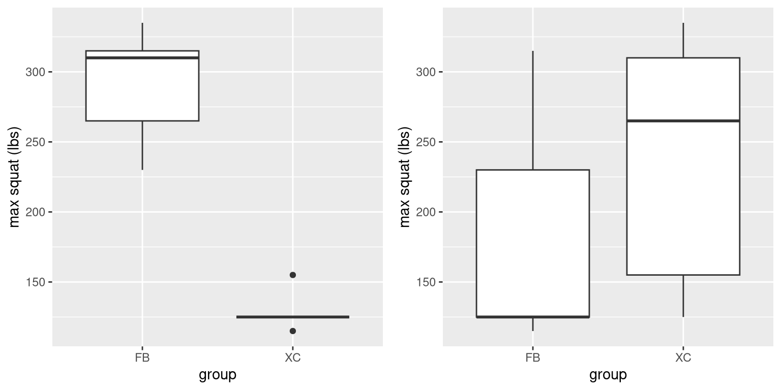
Figure 9.4: Left: Box plots of simulated squatting ability for football players and cross-country runners.Right: Box plots for subjects assigned to each group after scrambling group labels.

From the plot on the left side of Figure 9.4 it’s clear that there is a large difference between the two groups. We can do a standard t-test to test our hypothesis; for this example we will use the t.test() command in R, which gives the following result:

## 
##  Welch Two Sample t-test
## 
## data:  squat by group
## t = 8, df = 5, p-value = 2e-04
## alternative hypothesis: true difference in means between group FB and group XC is greater than 0
## 95 percent confidence interval:
##  121 Inf
## sample estimates:
## mean in group FB mean in group XC 
##              291              129

If we look at the p-value reported here, we see that the likelihood of such a difference under the null hypothesis is very small, using the t distribution to define the null.

Now let’s see how we could answer the same question using randomization. The basic idea is that if the null hypothesis of no difference between groups is true, then it shouldn’t matter which group one comes from (football players versus cross-country runners) – thus, to create data that are like our actual data but also conform to the null hypothesis, we can randomly reorder the data for the individuals in the dataset, and then recompute the difference between the groups. The results of such a shuffle are shown in the column labeled “shuffleSquat” in Table 9.2, and the boxplots of the resulting data are in the right panel of Figure 9.4.

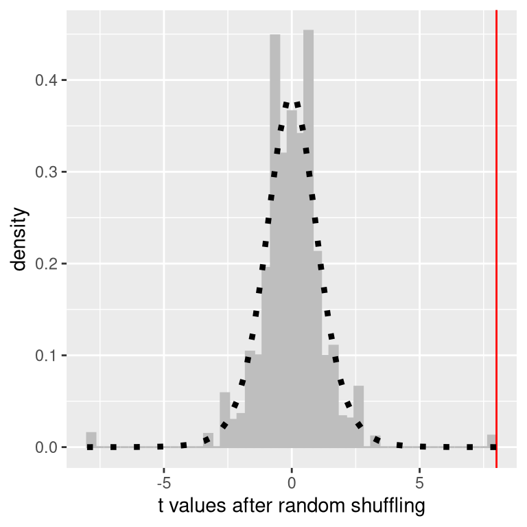
Figure 9.5: Histogram of t-values for the difference in means between the football and cross-country groups after randomly shuffling group membership. The vertical line denotes the actual difference observed between the two groups, and the dotted line shows the theoretical t distribution for this analysis.

After scrambling the data, we see that the two groups are now much more similar, and in fact the cross-country group now has a slightly higher mean. Now let’s do that 10000 times and store the t statistic for each iteration; if you are doing this on your own computer, it will take a moment to complete. Figure 9.5 shows the histogram of the t values across all of the random shuffles. As expected under the null hypothesis, this distribution is centered at zero (the mean of the distribution is 0.007). From the figure we can also see that the distribution of t values after shuffling roughly follows the theoretical t distribution under the null hypothesis (with mean=0), showing that randomization worked to generate null data. We can compute the p-value from the randomized data by measuring how many of the shuffled values are at least as extreme as the observed value: p(t > 8.01, df = 8) using randomization = 0.00410. This p-value is very similar to the p-value that we obtained using the t distribution, and both are quite extreme, suggesting that the observed data are very unlikely to have arisen if the null hypothesis is true - and in this case we know that it’s not true, because we generated the data.

9.3.5.4.1 Randomization: BMI/activity example

Now let’s use randomization to compute the p-value for the BMI/activity example. In this case, we will randomly shuffle the PhysActive variable and compute the difference between groups after each shuffle, and then compare our observed t statistic to the distribution of t statistics from the shuffled datasets. Figure 9.6 shows the distribution of t values from the shuffled samples, and we can also compute the probability of finding a value as large or larger than the observed value. The p-value obtained from randomization (0.000000) is very similar to the one obtained using the t distribution (0.000075). The advantage of the randomization test is that it doesn’t require that we assume that the data from each of the groups are normally distributed, though the t-test is generally quite robust to violations of that assumption. In addition, the randomization test can allow us to compute p-values for statistics when we don’t have a theoretical distribution like we do for the t-test.

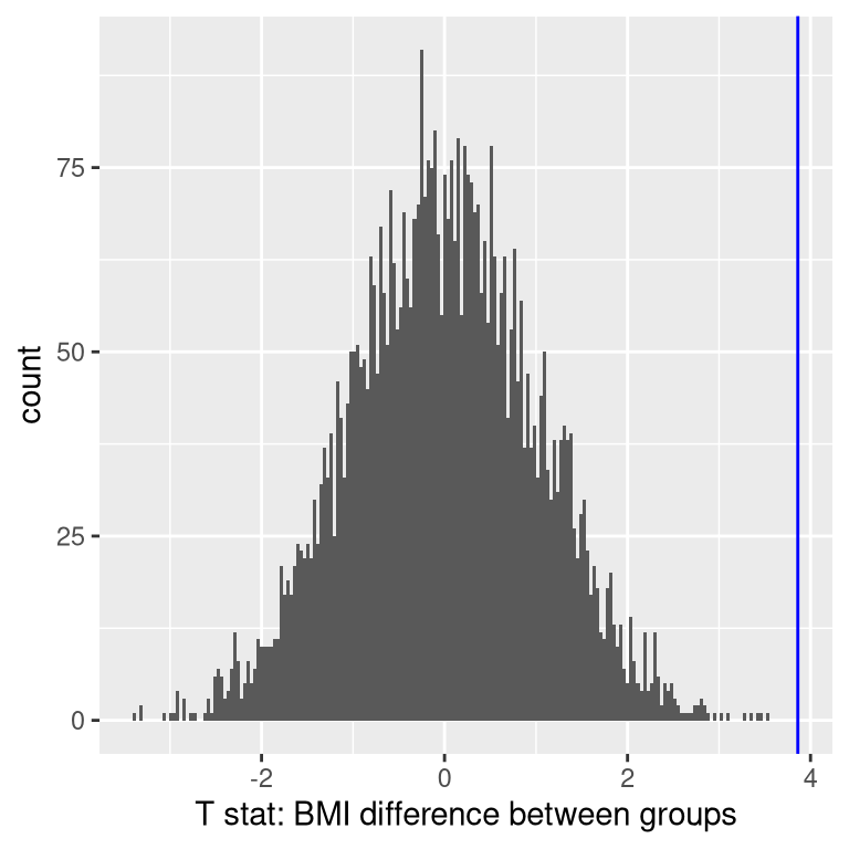
Figure 9.6: Histogram of t statistics after shuffling of group labels, with the observed value of the t statistic shown in the vertical line, and values at least as extreme as the observed value shown in lighter gray

We do have to make one main assumption when we use the randomization test, which we refer to as exchangeability. This means that all of the observations are distributed in the same way, such that we can interchange them without changing the overall distribution. The main place where this can break down is when there are related observations in the data; for example, if we had data from individuals in 4 different families, then we couldn’t assume that individuals were exchangeable, because siblings would be closer to each other than they are to individuals from other families. In general, if the data were obtained by random sampling, then the assumption of exchangeability should hold.

9.3.6 Step 6: Assess the “statistical significance” of the result

The next step is to determine whether the p-value that results from the previous step is small enough that we are willing to reject the null hypothesis and conclude instead that the alternative is true. How much evidence do we require? This is one of the most controversial questions in statistics, in part because it requires a subjective judgment – there is no “correct” answer.

Historically, the most common answer to this question has been that we should reject the null hypothesis if the p-value is less than 0.05. This comes from the writings of Ronald Fisher, who has been referred to as “the single most important figure in 20th century statistics” (Efron 1998):

“If P is between .1 and .9 there is certainly no reason to suspect the hypothesis tested. If it is below .02 it is strongly indicated that the hypothesis fails to account for the whole of the facts. We shall not often be astray if we draw a conventional line at .05 … it is convenient to draw the line at about the level at which we can say: Either there is something in the treatment, or a coincidence has occurred such as does not occur more than once in twenty trials” (R. A. Fisher 1925)

However, Fisher never intended \(p < 0.05\) to be a fixed rule:

“no scientific worker has a fixed level of significance at which from year to year, and in all circumstances, he rejects hypotheses; he rather gives his mind to each particular case in the light of his evidence and his ideas” (Ronald Aylmer Fisher 1956)

Instead, it is likely that p < .05 became a ritual due to the reliance upon tables of p-values that were used before computing made it easy to compute p values for arbitrary values of a statistic. All of the tables had an entry for 0.05, making it easy to determine whether one’s statistic exceeded the value needed to reach that level of significance.

The choice of statistical thresholds remains deeply controversial, and recently (Benjamin et al., 2018) it has been proposed that the default threshold be changed from .05 to .005, making it substantially more stringent and thus more difficult to reject the null hypothesis. In large part this move is due to growing concerns that the evidence obtained from a significant result at \(p < .05\) is relatively weak; we will return to this in our later discussion of reproducibility in Chapter 18.

9.3.6.1 Hypothesis testing as decision-making: The Neyman-Pearson approach

Whereas Fisher thought that the p-value could provide evidence regarding a specific hypothesis, the statisticians Jerzy Neyman and Egon Pearson disagreed vehemently. Instead, they proposed that we think of hypothesis testing in terms of its error rate in the long run:

“no test based upon a theory of probability can by itself provide any valuable evidence of the truth or falsehood of a hypothesis. But we may look at the purpose of tests from another viewpoint. Without hoping to know whether each separate hypothesis is true or false, we may search for rules to govern our behaviour with regard to them, in following which we insure that, in the long run of experience, we shall not often be wrong” (J. Neyman and Pearson 1933)

That is: We can’t know which specific decisions are right or wrong, but if we follow the rules, we can at least know how often our decisions will be wrong in the long run.

To understand the decision making framework that Neyman and Pearson developed, we first need to discuss statistical decision making in terms of the kinds of outcomes that can occur. There are two possible states of reality (\(H_0\) is true, or \(H_0\) is false), and two possible decisions (reject \(H_0\), or retain \(H_0\)). There are two ways in which we can make a correct decision:

• We can reject \(H_0\) when it is false (in the language of signal detection theory, we call this a hit)
• We can retain \(H_0\) when it is true (somewhat confusingly in this context, this is called a correct rejection)

There are also two kinds of errors we can make:

• We can reject \(H_0\) when it is actually true (we call this a false alarm, or Type I error)
• We can retain \(H_0\) when it is actually false (we call this a miss, or Type II error)

Neyman and Pearson coined two terms to describe the probability of these two types of errors in the long run:

• P(Type I error) = \(\alpha\)
• P(Type II error) = \(\beta\)

That is, if we set \(\alpha\) to .05, then in the long run we should make a Type I error 5% of the time. Whereas it’s common to set \(\alpha\) as .05, the standard value for an acceptable level of \(\beta\) is .2 - that is, we are willing to accept that 20% of the time we will fail to detect a true effect when it truly exists. We will return to this later when we discuss statistical power in Section 10.3, which is the complement of Type II error.

9.3.7 What does a significant result mean?

There is a great deal of confusion about what p-values actually mean (Gigerenzer, 2004). Let’s say that we do an experiment comparing the means between conditions, and we find a difference with a p-value of .01. There are a number of possible interpretations that one might entertain.

9.3.7.1 Does it mean that the probability of the null hypothesis being true is .01?

No. Remember that in null hypothesis testing, the p-value is the probability of the data given the null hypothesis (\(P(data|H_0)\)). It does not warrant conclusions about the probability of the null hypothesis given the data (\(P(H_0|data)\)). We will return to this question when we discuss Bayesian inference in a later chapter, as Bayes theorem lets us invert the conditional probability in a way that allows us to determine the probability of the hypothesis given the data.

9.3.7.2 Does it mean that the probability that you are making the wrong decision is .01?

No. This would be \(P(H_0|data)\), but remember as above that p-values are probabilities of data under \(H_0\), not probabilities of hypotheses.

9.3.7.3 Does it mean that if you ran the study again, you would obtain the same result 99% of the time?

No. The p-value is a statement about the likelihood of a particular dataset under the null; it does not allow us to make inferences about the likelihood of future events such as replication.

9.3.7.4 Does it mean that you have found a practically important effect?

No. There is an essential distinction between statistical significance and practical significance. As an example, let’s say that we performed a randomized controlled trial to examine the effect of a particular diet on body weight, and we find a statistically significant effect at p<.05. What this doesn’t tell us is how much weight was actually lost, which we refer to as the effect size (to be discussed in more detail in Chapter 10). If we think about a study of weight loss, then we probably don’t think that the loss of one ounce (i.e. the weight of a few potato chips) is practically significant. Let’s look at our ability to detect a significant difference of 1 ounce as the sample size increases.

Figure 9.7 shows how the proportion of significant results increases as the sample size increases, such that with a very large sample size (about 262,000 total subjects), we will find a significant result in more than 90% of studies when there is a 1 ounce difference in weight loss between the diets. While these are statistically significant, most physicians would not consider a weight loss of one ounce to be practically or clinically significant. We will explore this relationship in more detail when we return to the concept of statistical power in Section 10.3, but it should already be clear from this example that statistical significance is not necessarily indicative of practical significance.

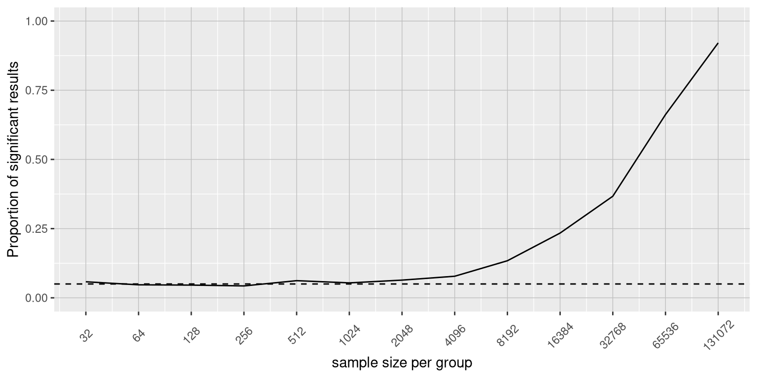
Figure 9.7: The proportion of signifcant results for a very small change (1 ounce, which is about .001 standard deviations) as a function of sample size.

9.4 NHST in a modern context: Multiple testing

So far we have discussed examples where we are interested in testing a single statistical hypothesis, and this is consistent with traditional science which often measured only a few variables at a time. However, in modern science we can often measure millions of variables per individual. For example, in genetic studies that quantify the entire genome, there may be many millions of measures per individual, and in the brain imaging research that my group does, we often collect data from more than 100,000 locations in the brain at once. When standard hypothesis testing is applied in these contexts, bad things can happen unless we take appropriate care.

Let’s look at an example to see how this might work. There is great interest in understanding the genetic factors that can predispose individuals to major mental illnesses such as schizophrenia, because we know that about 80% of the variation between individuals in the presence of schizophrenia is due to genetic differences. The Human Genome Project and the ensuing revolution in genome science has provided tools to examine the many ways in which humans differ from one another in their genomes. One approach that has been used in recent years is known as a genome-wide association study (GWAS), in which the genome of each individual is characterized at one million or more places to determine which letters of the genetic code they have at each location, focusing on locations where humans tend to differ frequently. After these have been determined, the researchers perform a statistical test at each location in the genome to determine whether people diagnosed with schizoprenia are more or less likely to have one specific version of the genetic sequence at that location.

Let’s imagine what would happen if the researchers simply asked whether the test was significant at p<.05 at each location, when in fact there is no true effect at any of the locations. To do this, we generate a large number of simulated t values from a null distribution, and ask how many of them are significant at p<.05. Let’s do this many times, and each time count up how many of the tests come out as significant (see Figure 9.8).

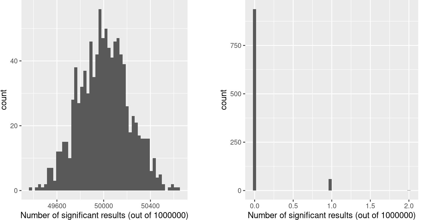
Figure 9.8: Left: A histogram of the number of significant results in each set of one million statistical tests, when there is in fact no true effect. Right: A histogram of the number of significant results across all simulation runs after applying the Bonferroni correction for multiple tests.

This shows that about 5% of all of the tests were significant in each run, meaning that if we were to use p < .05 as our threshold for statistical significance, then even if there were no truly significant relationships present, we would still “find” about 500 genes that were seemingly significant in each study (the expected number of significant results is simply \(n * \alpha\)). That is because while we controlled for the error per test, we didn’t control the error rate across our entire family of tests (known as the familywise error), which is what we really want to control if we are going to be looking at the results from a large number of tests. Using p<.05, our familywise error rate in the above example is one – that is, we are pretty much guaranteed to make at least one error in any particular study.

A simple way to control for the familywise error is to divide the alpha level by the number of tests; this is known as the Bonferroni correction, named after the Italian statistician Carlo Bonferroni. Using the data from our example above, we see in Figure 9.8 that only about 5 percent of studies show any significant results using the corrected alpha level of 0.000005 instead of the nominal level of .05. We have effectively controlled the familywise error, such that the probability of making any errors in our study is controlled at right around .05.

9.5 Learning objectives

• Identify the components of a hypothesis test, including the parameter of interest, the null and alternative hypotheses, and the test statistic.
• Describe the proper interpretations of a p-value as well as common misinterpretations
• Distinguish between the two types of error in hypothesis testing, and the factors that determine them.
• Describe how resampling can be used to compute a p-value.
• Describe the problem of multiple testing, and how it can be addressed
• Describe the main criticisms of null hypothesis statistical testing

9.6 Suggested readings

• Mindless Statistics, by Gerd Gigerenzer

References

Efron, Bradley. 1998. “R. A. Fisher in the 21st Century (Invited Paper Presented at the 1996 r. A. Fisher Lecture).” Statist. Sci. 13 (2): 95–122. https://doi.org/10.1214/ss/1028905930.

Fisher, R. A. 1925. Statistical Methods for Research Workers. Edinburgh Oliver & Boyd.

Fisher, Ronald Aylmer. 1956. Statistical Methods and Scientific Inference. New York: Hafner Pub. Co.

Neyman, J., and K. Pearson. 1933. “On the Problem of the Most Efficient Tests of Statistical Hypotheses.” Philosophical Transactions of the Royal Society of London A: Mathematical, Physical and Engineering Sciences 231 (694-706): 289–337. https://doi.org/10.1098/rsta.1933.0009.