Chapter 7 Sampling
One of the foundational ideas in statistics is that we can make inferences about an entire population based on a relatively small sample of individuals from that population. In this chapter we will introduce the concept of statistical sampling and discuss why it works.
Anyone living in the United States will be familiar with the concept of sampling from the political polls that have become a central part of our electoral process. In some cases, these polls can be incredibly accurate at predicting the outcomes of elections. The best known example comes from the 2008 and 2012 US Presidential elections, when the pollster Nate Silver correctly predicted electoral outcomes for 49/50 states in 2008 and for all 50 states in 2012. Silver did this by combining data from 21 different polls, which vary in the degree to which they tend to lean towards either the Republican or Democratic side. Each of these polls included data from about 1000 likely voters – meaning that Silver was able to almost perfectly predict the pattern of votes of more than 125 million voters using data from only about 21,000 people, along with other knowledge (such as how those states have voted in the past).
7.1 How do we sample?
Our goal in sampling is to determine the value of a statistic for an entire population of interest, using just a small subset of the population. We do this primarily to save time and effort – why go to the trouble of measuring every individual in the population when just a small sample is sufficient to accurately estimate the statistic of interest?
In the election example, the population is all registered voters in the region being polled, and the sample is the set of 1000 individuals selected by the polling organization. The way in which we select the sample is critical to ensuring that the sample is representative of the entire population, which is a main goal of statistical sampling. It’s easy to imagine a non-representative sample; if a pollster only called individuals whose names they had received from the local Democratic party, then it would be unlikely that the results of the poll would be representative of the population as a whole. In general, we would define a representative poll as being one in which every member of the population has an equal chance of being selected. When this fails, then we have to worry about whether the statistic that we compute on the sample is biased - that is, whether its value is systematically different from the population value (which we refer to as a parameter). Keep in mind that we generally don’t know this population parameter, because if we did then we wouldn’t need to sample! But we will use examples where we have access to the entire population, in order to explain some of the key ideas.
It’s important to also distinguish between two different ways of sampling: with replacement versus without replacement. In sampling with replacement, after a member of the population has been sampled, they are put back into the pool so that they can potentially be sampled again. In sampling without replacement, once a member has been sampled they are not eligible to be sampled again. It’s most common to use sampling without replacement, but there will be some contexts in which we will use sampling with replacement, as when we discuss a technique called bootstrapping in Chapter 8.
7.2 Sampling error
Regardless of how representative our sample is, it’s likely that the statistic that we compute from the sample is going to differ at least slightly from the population parameter. We refer to this as sampling error. If we take multiple samples, the value of our statistical estimate will also vary from sample to sample; we refer to this distribution of our statistic across samples as the sampling distribution.
Sampling error is directly related to the quality of our measurement of the population. Clearly we want the estimates obtained from our sample to be as close as possible to the true value of the population parameter. However, even if our statistic is unbiased (that is, we expect it to have the same value as the population parameter), the value for any particular estimate will differ from the population value, and those differences will be greater when the sampling error is greater. Thus, reducing sampling error is an important step towards better measurement.
We will use the NHANES dataset as an example; we are going to assume that the NHANES dataset is the entire population of interest, and then we will draw random samples from this population. We will have more to say in the next chapter about exactly how the generation of “random” samples works in a computer.
In this example, we know the adult population mean (168.35) and standard deviation (10.16) for height because we are assuming that the NHANES dataset is the population. Table 7.1 shows the statistics computed from a few samples of 50 individuals from the NHANES population.
| sampleMean | sampleSD |
|---|---|
| 167 | 9.1 |
| 171 | 8.3 |
| 170 | 10.6 |
| 166 | 9.5 |
| 168 | 9.5 |
The sample mean and standard deviation are similar but not exactly equal to the population values. Now let’s take a large number of samples of 50 individuals, compute the mean for each sample, and look at the resulting sampling distribution of means. We have to decide how many samples to take in order to do a good job of estimating the sampling distribution – in this case we will take 5000 samples so that we are very confident in the answer. Note that simulations like this one can sometimes take a few minutes to run, and might make your computer huff and puff. The histogram in Figure 7.1 shows that the means estimated for each of the samples of 50 individuals vary somewhat, but that overall they are centered around the population mean. The average of the 5000 sample means (168.3463) is very close to the true population mean (168.3497).
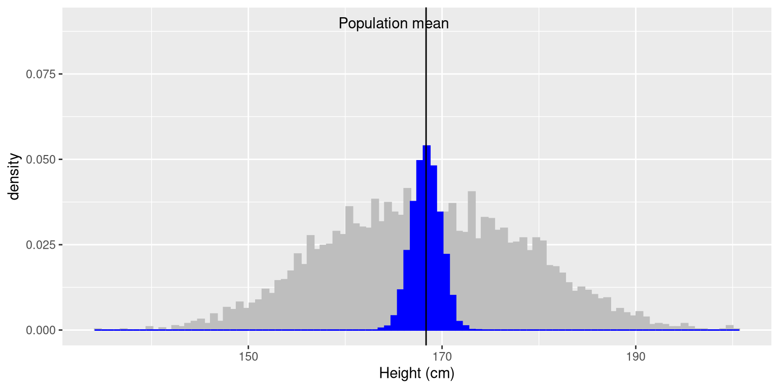
Figure 7.1: The blue histogram shows the sampling distribution of the mean over 5000 random samples from the NHANES dataset. The histogram for the full dataset is shown in gray for reference.
7.3 Standard error of the mean
Later in the book it will become essential to be able to characterize how variable our samples are, in order to make inferences about the sample statistics. For the mean, we do this using a quantity called the standard error of the mean (SEM), which one can think of as the standard deviation of the sampling distribution of the mean. To compute the standard error of the mean for our sample, we divide the estimated standard deviation by the square root of the sample size:
\[ SEM = \frac{\hat{\sigma}}{\sqrt{n}} \]
Note that we have to be careful about computing SEM using the estimated standard deviation if our sample is small (less than about 30).
Because we have many samples from the NHANES population and we actually know the population SEM (which we compute by dividing the population standard deviation by the size of the population), we can confirm that the SEM computed using the population parameter (1.44) is very close to the observed standard deviation of the means for the samples that we took from the NHANES dataset (1.43).
The formula for the standard error of the mean implies that the quality of our measurement involves two quantities: the population variability, and the size of our sample. Because the sample size is the denominator in the formula for SEM, a larger sample size will yield a smaller SEM when holding the population variability constant. We have no control over the population variability, but we do have control over the sample size. Thus, if we wish to improve our sample statistics (by reducing their sampling variability) then we should use larger samples. However, the formula also tells us something very fundamental about statistical sampling – namely, that the utility of larger samples diminishes with the square root of the sample size. This means that doubling the sample size will not double the quality of the statistics; rather, it will improve it by a factor of \(\sqrt{2}\). In Section 10.3 we will discuss statistical power, which is intimately tied to this idea.
7.4 The Central Limit Theorem
The Central Limit Theorem tells us that as sample sizes get larger, the sampling distribution of the mean will become normally distributed, even if the data within each sample are not normally distributed.
First, let’s say a little bit about the normal distribution. It’s also known as the Gaussian distribution, after Carl Friedrich Gauss, a mathematician who didn’t invent it but played a role in its development. The normal distribution is described in terms of two parameters: the mean (which you can think of as the location of the peak), and the standard deviation (which specifies the width of the distribution). The bell-like shape of the distribution never changes, only its location and width. The normal distribution is commonly observed in data collected in the real world, as we have already seen in Chapter 3 — and the central limit theorem gives us some insight into why that occurs.
To see the central limit theorem in action, let’s work with the variable AlcoholYear from the NHANES dataset, which is highly skewed, as shown in the left panel of Figure 7.2. This distribution is, for lack of a better word, funky – and definitely not normally distributed. Now let’s look at the sampling distribution of the mean for this variable. Figure 7.2 shows the sampling distribution for this variable, which is obtained by repeatedly drawing samples of size 50 from the NHANES dataset and taking the mean. Despite the clear non-normality of the original data, the sampling distribution is remarkably close to the normal.
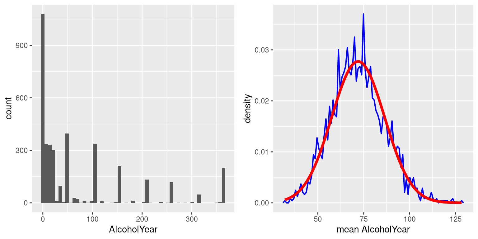
Figure 7.2: Left: Distribution of the variable AlcoholYear in the NHANES dataset, which reflects the number of days that the individual drank in a year. Right: The sampling distribution of the mean for AlcoholYear in the NHANES dataset, obtained by drawing repeated samples of size 50, in blue. The normal distribution with the same mean and standard deviation is shown in red.
The Central Limit Theorem is important for statistics because it allows us to safely assume that the sampling distribution of the mean will be normal in most cases. This means that we can take advantage of statistical techniques that assume a normal distribution, as we will see in the next section. It’s also important because it tells us why normal distributions are so common in the real world; any time we combine many different factors into a single number, the result is likely to be a normal distribution. For example, the height of any adult depends on a complex mixture of their genetics and experience; even if those individual contributions may not be normally distributed, when we combine them the result is a normal distribution.
7.5 Learning objectives
Having read this chapter, you should be able to:
- Distinguish between a population and a sample, and between population parameters and sample statistics
- Describe the concepts of sampling error and sampling distribution
- Compute the standard error of the mean
- Describe how the Central Limit Theorem determines the nature of the sampling distribution of the mean