Chapter 3: Summarizing data

import pandas as pd
import sidetable
import numpy as np
import matplotlib.pyplot as plt
import seaborn as sns
from scipy.stats import norm


import rpy2.robjects as ro
from rpy2.robjects.packages import importr
from rpy2.robjects import pandas2ri
pandas2ri.activate()
from rpy2.robjects.conversion import localconverter
# import NHANES package
base = importr('NHANES')

with localconverter(ro.default_converter + pandas2ri.converter):
  NHANES = ro.conversion.rpy2py(ro.r['NHANES'])

 
NHANES = NHANES.drop_duplicates(subset='ID')

Table 3.1

pd.DataFrame(NHANES.PhysActive.value_counts(dropna=False))

	PhysActive
Yes	2972
No	2473
NaN	1334

Table 3.2

table_df = NHANES.stb.freq(['PhysActive']).drop(
    ['cumulative_count', 'cumulative_percent'], axis=1)
table_df['RelativeFrequency'] = table_df.percent / 100
table_df = table_df.rename(columns={
    'count': 'AbsoluteFrequency',
    'percent': 'Percentage'})
table_df.style.hide(axis="index")

PhysActive	AbsoluteFrequency	Percentage	RelativeFrequency
Yes	2972	54.582185	0.545822
No	2473	45.417815	0.454178

Table 3.3

NHANES_sleep = NHANES.query('SleepHrsNight > 0')
table_df = NHANES_sleep.stb.freq(
    ['SleepHrsNight'])
table_df['RelativeFrequency'] = table_df.percent / 100
table_df = table_df.rename(columns={
    'count': 'AbsoluteFrequency',
    'percent': 'Percentage'}).sort_values(by='SleepHrsNight').drop(
    ['cumulative_count', 'cumulative_percent'], axis=1)

table_df.style.hide(axis="index")

SleepHrsNight	AbsoluteFrequency	Percentage	RelativeFrequency
2	9	0.178749	0.001787
3	49	0.973188	0.009732
4	200	3.972195	0.039722
5	406	8.063555	0.080636
6	1172	23.277061	0.232771
7	1394	27.686197	0.276862
8	1405	27.904667	0.279047
9	271	5.382324	0.053823
10	97	1.926514	0.019265
11	15	0.297915	0.002979
12	17	0.337637	0.003376

Figure 3.2

fig, ax = plt.subplots(1, 2, figsize=(12,8))

sns.histplot(NHANES_sleep.SleepHrsNight, ax=ax[0], discrete=True)
sns.histplot(NHANES_sleep.SleepHrsNight, ax=ax[1], stat='density', discrete=True)

<Axes: xlabel='SleepHrsNight', ylabel='Density'>

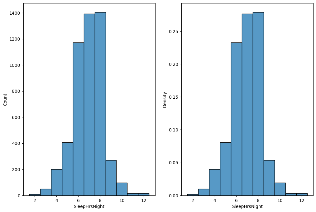
Figure 3.3

fig, ax = plt.subplots(1, 2, figsize=(12,8))

sns.histplot(NHANES_sleep.SleepHrsNight, ax=ax[0],
             element="step", fill=False, cumulative=True, )
sns.histplot(NHANES_sleep.SleepHrsNight,  ax=ax[0], discrete=True)

sns.histplot(NHANES_sleep.SleepHrsNight, ax=ax[1], stat='density',
             element="step", fill=False, cumulative=True, )
sns.histplot(NHANES_sleep.SleepHrsNight, ax=ax[1], stat='density', discrete=True)

<Axes: xlabel='SleepHrsNight', ylabel='Density'>

Figure 3.4

fig, ax = plt.subplots(1, 2, figsize=(12,8))

sns.histplot(NHANES.Age, binwidth=1, ax=ax[0])

sns.histplot(NHANES.Height, binwidth=1, ax=ax[1])

<Axes: xlabel='Height', ylabel='Count'>

Figure 3.5

fig, ax = plt.subplots(2, 2, figsize=(12,8))

NHANES['isChild'] = NHANES.Age < 18
NHANES_adult = NHANES.dropna(subset=['Age', 'Height']).query('Age > 17')

sns.histplot(NHANES, x='Height', hue='isChild', binwidth=1, ax=ax[0][0])
ax[0][0].set_title('A. All individuals')

sns.histplot(NHANES_adult, x='Height',  binwidth=1, ax=ax[0][1])
ax[0][0].set_title('B. Adults only')

sns.histplot(NHANES_adult, x='Height',  binwidth=.1, ax=ax[1][0])
ax[1][0].set_title('B. Adults only (bin width=.1)')

Text(0.5, 1.0, 'B. Adults only (bin width=.1)')

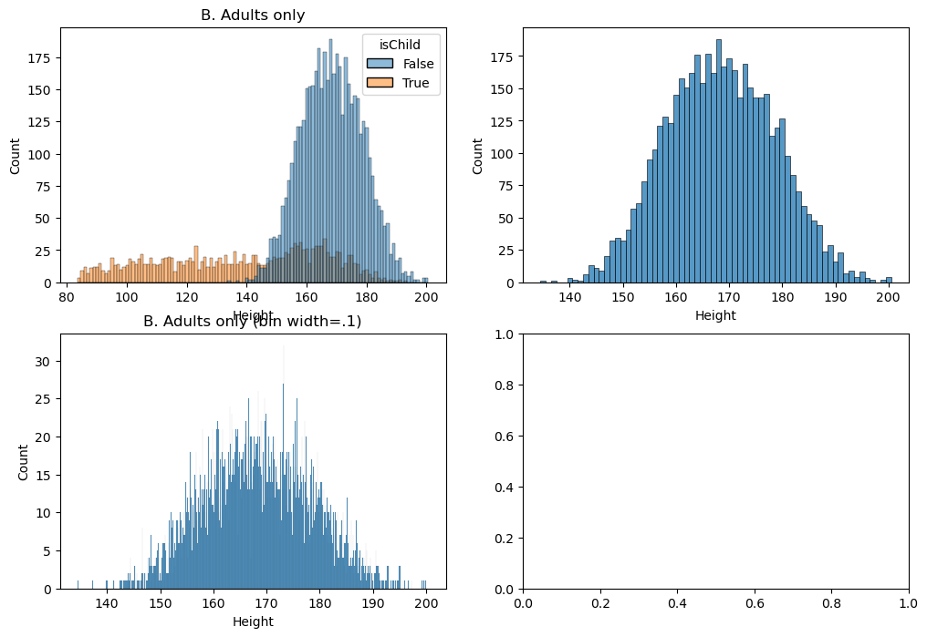
Table 3.5

NHANES_adult['Height'][44:50]

96     169.6
97     169.8
101    167.5
102    155.2
104    173.8
107    174.5
Name: Height, dtype: float64

Figure 3.6

# first update the summary to include the mean and standard deviation of each
# dataset
# NOTE: some NA values get turned into large negative numbers in the conversion from R, so remove those

pulsedata = NHANES_adult.dropna(subset=['Pulse']).query('Pulse > 0')[['Pulse']]
heightdata = NHANES_adult.dropna(subset=['Height']).query('Height > 0')[['Height']]

pulse_summary = pulsedata.describe()
pulse_summary.loc['binwidth'] = np.diff(np.histogram_bin_edges(pulsedata.Pulse, 'fd'))[0]

height_summary = heightdata.describe()
height_summary.loc['binwidth'] = np.diff(np.histogram_bin_edges(heightdata.Height, 'fd'))[0]

heightDist = pd.DataFrame({'x': np.arange(height_summary.loc['min'][0], height_summary.loc['max'][0], .1)})
heightDist['norm'] = norm.pdf(
    heightDist.x, height_summary.loc['mean'][0], height_summary.loc['std'])

pulseDist = pd.DataFrame({'x': np.arange(pulse_summary.loc['min'][0], pulse_summary.loc['max'][0], .1)})
pulseDist['norm'] = norm.pdf(
    pulseDist.x, pulse_summary.loc['mean'][0], pulse_summary.loc['std'])

fig, ax = plt.subplots(1, 2, figsize=(12,8))

sns.histplot(heightdata.Height, stat='density', binwidth=height_summary.loc['binwidth'][0], color='gray', ax=ax[0])
ax[0].plot(heightDist.x, heightDist.norm, lw=2, color='b')

sns.histplot(pulsedata.Pulse, stat='density', binwidth=pulse_summary.loc['binwidth'][0], color='gray', ax=ax[1])
ax[1].plot(pulseDist.x, pulseDist.norm, lw=2, color='b')

[<matplotlib.lines.Line2D at 0x7f56a7c1d930>]

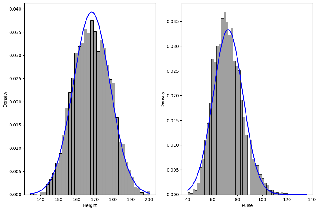
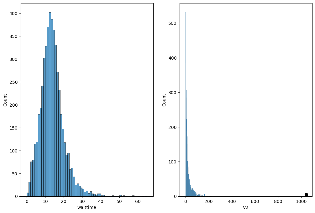
Figure 3.7

waittimes = pd.read_csv('https://raw.githubusercontent.com/statsthinking21/statsthinking21-figures-data/main/04/sfo_wait_times_2017.csv')

fig, ax = plt.subplots(1, 2, figsize=(12,8))
sns.histplot(waittimes.waittime, binwidth=1, ax=ax[0])

fbdata = pd.read_csv('https://raw.githubusercontent.com/statsthinking21/statsthinking21-figures-data/main/04/facebook_combined.txt', names=['V1', 'V2'], delimiter=' ')
friends_table = fbdata.groupby('V1').count()
sns.histplot(friends_table.V2, binwidth=2, ax=ax[1])
plt.plot([friends_table.max()['V2']], [5], marker='.', markersize=14, color='k')

[<matplotlib.lines.Line2D at 0x7f56a6236e00>]