Chapter 14: The General Linear Model
Contents
Chapter 14: The General Linear Model#
import pandas as pd
import numpy as np
import matplotlib.pyplot as plt
import seaborn as sns
from scipy.stats import norm, t, binom, scoreatpercentile
import pingouin as pg
import matplotlib
import statsmodels.api as sm
import statsmodels.formula.api as smf
from sklearn.metrics import r2_score, mean_squared_error
from sklearn.model_selection import KFold

import rpy2.robjects as ro
from rpy2.robjects.packages import importr
from rpy2.robjects import pandas2ri
pandas2ri.activate()
from rpy2.robjects.conversion import localconverter
# import NHANES package
base = importr('NHANES')
%load_ext rpy2.ipython

with localconverter(ro.default_converter + pandas2ri.converter):
  NHANES = ro.conversion.rpy2py(ro.r['NHANES'])


NHANES = NHANES.drop_duplicates(subset='ID')
NHANES_adult = NHANES.dropna(subset=['Weight']).query('Age > 17 and BPSysAve > 0')

rng = np.random.default_rng(1234567)
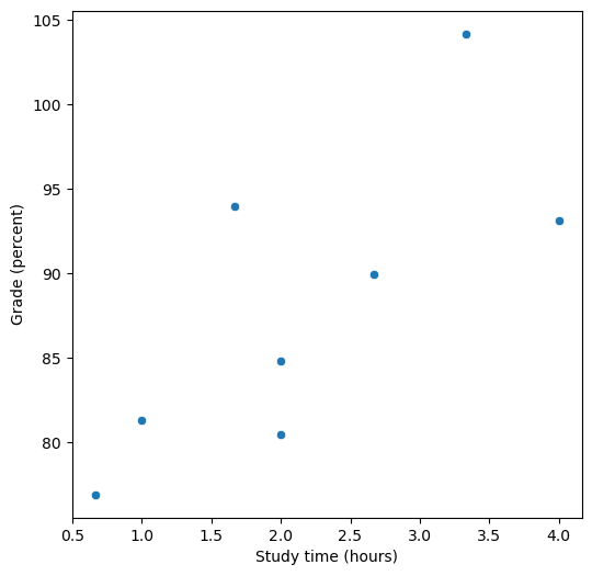
Figure 14.1#
# Data differ from book example because y values are random samples
betas = np.array([6, 5])

df = pd.DataFrame({'studyTime': np.array([2, 3, 5, 6, 6, 8, 10, 12]) / 3,
                   'priorClass': [0, 1, 1, 0, 1, 0, 1, 0]})
grade_intercept = 70
df['grade'] = df.values.dot(betas) + rng.normal(size=8, loc = grade_intercept, scale = 5)

fig = plt.figure(figsize=(6,6))
sns.scatterplot(data=df, x='studyTime', y='grade')
plt.xlabel('Study time (hours)')
plt.ylabel('Grade (percent)')
Text(0, 0.5, 'Grade (percent)')
Correlation test#
# compute correlation between grades and study time
corTestResult = pg.corr(df['studyTime'], df['grade'])
corTestResult
| n | r | CI95% | p-val | BF10 | power | |
|---|---|---|---|---|---|---|
| pearson | 8 | 0.742254 | [0.08, 0.95] | 0.034959 | 2.886 | 0.612544 |
Figure 14.2#
mod = smf.ols(formula='grade ~ studyTime', data=df)
res = mod.fit()

fig = plt.figure(figsize=(6,6))
plt.xlim([-0.5, 4.5])
sns.regplot(data=df, x='studyTime', y='grade', color='black',
            line_kws={'color': 'blue'}, ci=None, truncate=False)
plt.xlabel('Study time (hours)')
plt.ylabel('Grade (percent)')
xmax = df.studyTime.max() * 1.1

plt.plot([2, 3], [res.params.dot(np.array([1, 2])), res.params.dot(np.array([1, 2]))], 'k', linestyle='dashed')
plt.plot([3, 3], [res.params.dot(np.array([1, 2])), res.params.dot(np.array([1, 3]))], 'k', linestyle='dashed')
plt.plot([0, xmax], [res.params['Intercept'], res.params['Intercept']], 'k:')
[<matplotlib.lines.Line2D at 0x7f3993c48730>]
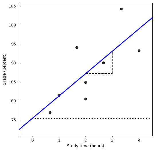
Table 14.1#
nstudents = 100

readingScores = pd.DataFrame({'test1': rng.normal(100, 10, nstudents),
                              'test2': rng.normal(100, 10, nstudents)})

cutoff = scoreatpercentile(readingScores.test1, 25)

readingScores[readingScores.test1 < cutoff].mean()
test1    87.084873
test2    99.249985
dtype: float64
Linear model output#
print(res.summary())
                            OLS Regression Results
==============================================================================
Dep. Variable:                  grade   R-squared:                       0.551
Model:                            OLS   Adj. R-squared:                  0.476
Method:                 Least Squares   F-statistic:                     7.361
Date:                Tue, 21 Feb 2023   Prob (F-statistic):             0.0350
Time:                        21:50:28   Log-Likelihood:                -25.157
No. Observations:                   8   AIC:                             54.31
Df Residuals:                       6   BIC:                             54.47
Df Model:                           1
Covariance Type:            nonrobust
==============================================================================
                 coef    std err          t      P>|t|      [0.025      0.975]
------------------------------------------------------------------------------
Intercept     75.3225      5.241     14.371      0.000      62.498      88.147
studyTime      5.9019      2.175      2.713      0.035       0.579      11.225
==============================================================================
Omnibus:                        1.336   Durbin-Watson:                   2.668
Prob(Omnibus):                  0.513   Jarque-Bera (JB):                0.897
Skew:                           0.672   Prob(JB):                        0.639
Kurtosis:                       2.060   Cond. No.                         6.30
==============================================================================

Notes:
[1] Standard Errors assume that the covariance matrix of the errors is correctly specified.
/opt/conda/lib/python3.10/site-packages/scipy/stats/_stats_py.py:1736: UserWarning: kurtosistest only valid for n>=20 ... continuing anyway, n=8
  warnings.warn("kurtosistest only valid for n>=20 ... continuing "
Linear regression output for study time and prior class#
mod2 = smf.ols(formula='grade ~ studyTime + priorClass', data=df)
res2 = mod2.fit()
print(res2.summary())
                            OLS Regression Results
==============================================================================
Dep. Variable:                  grade   R-squared:                       0.780
Model:                            OLS   Adj. R-squared:                  0.693
Method:                 Least Squares   F-statistic:                     8.889
Date:                Tue, 21 Feb 2023   Prob (F-statistic):             0.0226
Time:                        21:50:28   Log-Likelihood:                -22.294
No. Observations:                   8   AIC:                             50.59
Df Residuals:                       5   BIC:                             50.83
Df Model:                           2
Covariance Type:            nonrobust
==============================================================================
                 coef    std err          t      P>|t|      [0.025      0.975]
------------------------------------------------------------------------------
Intercept     69.9340      4.655     15.024      0.000      57.969      81.899
studyTime      6.5119      1.687      3.860      0.012       2.175      10.849
priorClass     8.1336      3.557      2.287      0.071      -1.010      17.277
==============================================================================
Omnibus:                        1.929   Durbin-Watson:                   2.521
Prob(Omnibus):                  0.381   Jarque-Bera (JB):                0.755
Skew:                          -0.126   Prob(JB):                        0.686
Kurtosis:                       1.517   Cond. No.                         7.91
==============================================================================

Notes:
[1] Standard Errors assume that the covariance matrix of the errors is correctly specified.
/opt/conda/lib/python3.10/site-packages/scipy/stats/_stats_py.py:1736: UserWarning: kurtosistest only valid for n>=20 ... continuing anyway, n=8
  warnings.warn("kurtosistest only valid for n>=20 ... continuing "
Figure 14.3#
fig = plt.figure(figsize=(6,6))
plt.xlim([-0.5, xmax])

sns.scatterplot(data=df, x='studyTime', y='grade', color='black', style='priorClass')
plt.xlabel('Study time (hours)')
plt.ylabel('Grade (percent)')
xmax = df.studyTime.max() * 1.1

plt.plot([0, xmax], [res2.params.dot(np.array([1, 0, 0])), res2.params.dot(np.array([1, xmax, 0]))], 'k')
plt.plot([0, xmax], [res2.params.dot(np.array([1, 0, 1])), res2.params.dot(np.array([1, xmax, 1]))], 'k', linestyle='dashed')
plt.plot([2, 2], [res2.params.dot(np.array([1, 2, 0])), res2.params.dot(np.array([1, 2, 1]))], 'k', linestyle='dotted')
[<matplotlib.lines.Line2D at 0x7f3993ba99c0>]
Figure 14.4#
fig, ax = plt.subplots(2, 2, figsize=(12,12))

df = pd.DataFrame({'group': [-1, 1] * 10,
                  'caffeine': rng.uniform(size=20) * 100})
df['speaking'] = 0.5 * df.caffeine * -df.group + 20 * df.group + rng.normal(size=20) * 10
df['anxiety'] = ['anxious' if i == 1 else 'notAnxious' for i in df.group]


# perform linear regression with caffeine as independent variable
res_caf = smf.ols(formula='speaking ~ caffeine', data=df).fit()

# compute linear regression adding anxiety to model
res_caf_anx = smf.ols(formula='speaking ~ caffeine + anxiety', data=df).fit()

# compute linear regression including caffeine X anxiety interaction
res_caf_anx_int = smf.ols(formula='speaking ~ caffeine * anxiety', data=df).fit()

sns.scatterplot(data=df, x='caffeine', y='speaking', ax=ax[0][0])

sns.scatterplot(data=df, x='caffeine', y='speaking', hue='anxiety', ax=ax[0][1])

sns.regplot(data=df.query('group == -1'), x='caffeine', y='speaking',  ax=ax[1][0], ci=None, truncate=False)
sns.regplot(data=df.query('group == 1'), x='caffeine', y='speaking',  ax=ax[1][0], ci=None, truncate=False)

ax[1][1].set_visible(False)
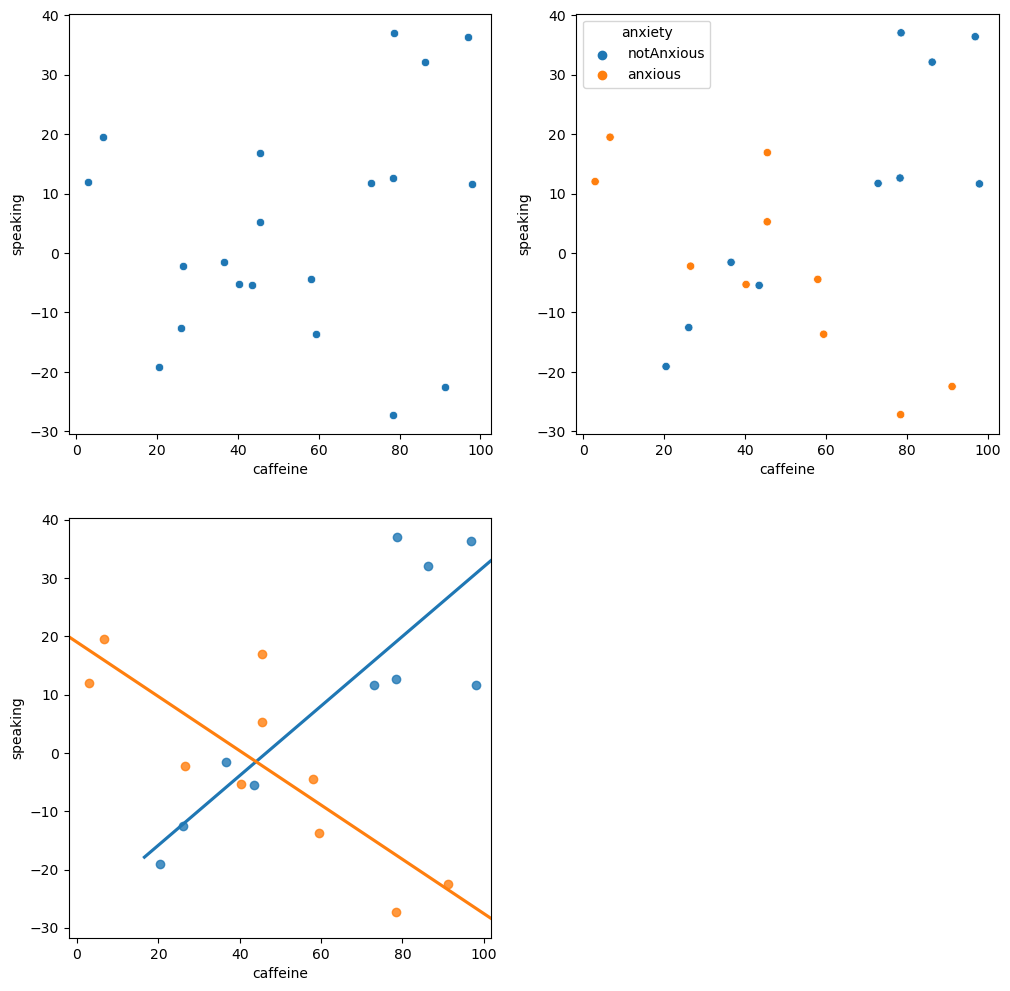
Linear model for caffeine#
print(res_caf.summary())
                            OLS Regression Results
==============================================================================
Dep. Variable:               speaking   R-squared:                       0.051
Model:                            OLS   Adj. R-squared:                 -0.001
Method:                 Least Squares   F-statistic:                    0.9718
Date:                Tue, 21 Feb 2023   Prob (F-statistic):              0.337
Time:                        21:50:29   Log-Likelihood:                -86.007
No. Observations:                  20   AIC:                             176.0
Df Residuals:                      18   BIC:                             178.0
Df Model:                           1
Covariance Type:            nonrobust
==============================================================================
                 coef    std err          t      P>|t|      [0.025      0.975]
------------------------------------------------------------------------------
Intercept     -3.7625      8.994     -0.418      0.681     -22.659      15.134
caffeine       0.1436      0.146      0.986      0.337      -0.162       0.450
==============================================================================
Omnibus:                        0.328   Durbin-Watson:                   2.223
Prob(Omnibus):                  0.849   Jarque-Bera (JB):                0.488
Skew:                          -0.133   Prob(JB):                        0.784
Kurtosis:                       2.283   Cond. No.                         132.
==============================================================================

Notes:
[1] Standard Errors assume that the covariance matrix of the errors is correctly specified.
Linear model result for caffeine and anxiety#
print(res_caf_anx.summary())
                            OLS Regression Results
==============================================================================
Dep. Variable:               speaking   R-squared:                       0.131
Model:                            OLS   Adj. R-squared:                  0.029
Method:                 Least Squares   F-statistic:                     1.283
Date:                Tue, 21 Feb 2023   Prob (F-statistic):              0.303
Time:                        21:50:29   Log-Likelihood:                -85.127
No. Observations:                  20   AIC:                             176.3
Df Residuals:                      17   BIC:                             179.2
Df Model:                           2
Covariance Type:            nonrobust
=========================================================================================
                            coef    std err          t      P>|t|      [0.025      0.975]
-----------------------------------------------------------------------------------------
Intercept                -5.9466      9.027     -0.659      0.519     -24.992      13.099
anxiety[T.notAnxious]    10.9220      8.732      1.251      0.228      -7.501      29.345
caffeine                  0.0836      0.151      0.552      0.588      -0.236       0.403
==============================================================================
Omnibus:                        2.592   Durbin-Watson:                   2.082
Prob(Omnibus):                  0.274   Jarque-Bera (JB):                1.151
Skew:                          -0.004   Prob(JB):                        0.562
Kurtosis:                       1.825   Cond. No.                         145.
==============================================================================

Notes:
[1] Standard Errors assume that the covariance matrix of the errors is correctly specified.
Linear model result for interaction#
print(res_caf_anx_int.summary())
                            OLS Regression Results
==============================================================================
Dep. Variable:               speaking   R-squared:                       0.761
Model:                            OLS   Adj. R-squared:                  0.716
Method:                 Least Squares   F-statistic:                     16.99
Date:                Tue, 21 Feb 2023   Prob (F-statistic):           3.14e-05
Time:                        21:50:29   Log-Likelihood:                -72.214
No. Observations:                  20   AIC:                             152.4
Df Residuals:                      16   BIC:                             156.4
Df Model:                           3
Covariance Type:            nonrobust
==================================================================================================
                                     coef    std err          t      P>|t|      [0.025      0.975]
--------------------------------------------------------------------------------------------------
Intercept                         18.9944      6.209      3.059      0.007       5.833      32.156
anxiety[T.notAnxious]            -46.7564     10.056     -4.650      0.000     -68.073     -25.439
caffeine                          -0.4655      0.118     -3.959      0.001      -0.715      -0.216
caffeine:anxiety[T.notAnxious]     1.0625      0.164      6.496      0.000       0.716       1.409
==============================================================================
Omnibus:                        1.060   Durbin-Watson:                   2.686
Prob(Omnibus):                  0.589   Jarque-Bera (JB):                0.367
Skew:                           0.328   Prob(JB):                        0.833
Kurtosis:                       3.103   Cond. No.                         367.
==============================================================================

Notes:
[1] Standard Errors assume that the covariance matrix of the errors is correctly specified.
Analysis of variance result#
print(sm.stats.anova_lm(res_caf_anx, res_caf_anx_int))
   df_resid          ssr  df_diff      ss_diff          F    Pr(>F)
0      17.0  5828.534062      0.0          NaN        NaN       NaN
1      16.0  1602.468696      1.0  4226.065367  42.195549  0.000007
Figure 14.5#
qq_df = pd.DataFrame({'norm': rng.normal(size=100),
                      'unif': rng.uniform(size=100)})

fig, ax = plt.subplots(1, 2, figsize=(12,6))

_ = sm.qqplot(qq_df['norm'], line ='45', ax=ax[0])
ax[0].set_title('Normal data')

_ = sm.qqplot(qq_df['unif'], line ='45', ax=ax[1])
ax[1].set_title('Non-normal data')
Text(0.5, 1.0, 'Non-normal data')
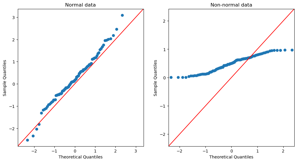
Table 14.2#
NHANES_child = NHANES.query('Age < 18')[['Height', 'Weight', 'TVHrsDayChild', 'HHIncomeMid', 'CompHrsDayChild', 'Age']].dropna()

# create function to sample data and compute regression on in-sample and out-of-sample data

def get_sample_predictions(sample_size=250, shuffle = False):
    # generate a sample from NHANES
    orig_sample = NHANES_child.sample(sample_size)

    # if shuffle is turned on, then randomly shuffle the weight variable
    if shuffle:
        orig_sample.Weight = rng.permuted(orig_sample.Weight)

    # compute the regression line for Weight, as a function of several
    # other variables (with all possible interactions between variables)
    heightRegressOrig = smf.ols(
        formula='Weight ~ Height * TVHrsDayChild * CompHrsDayChild * HHIncomeMid * Age',
        data=orig_sample).fit()

    # compute the predictions
    pred_orig = heightRegressOrig.predict(orig_sample)


    # create a new sample from the same population
    new_sample = NHANES_child.sample(sample_size)

    # use the model fom the original sample to predict the
    # Weight values for the new sample
    pred_new = heightRegressOrig.predict(new_sample)

    # return r-squared and rmse for original and new data
    return([
        r2_score(pred_orig, orig_sample.Weight),
        r2_score(pred_new, new_sample.Weight),
        np.sqrt(mean_squared_error(pred_orig, orig_sample.Weight)),
        np.sqrt(mean_squared_error(pred_new, new_sample.Weight))])


# implement the function
nruns = 100
sim_results = pd.DataFrame([get_sample_predictions() for i in range(nruns)],
                           columns=['r2_orig', 'r2_new', 'RMSE_orig', 'RMSE_new'])
sim_results_shuffled = pd.DataFrame([get_sample_predictions(shuffle=True) for i in range(nruns)],
                           columns=['r2_orig', 'r2_new', 'RMSE_orig', 'RMSE_new'])

sim_results_combined = pd.DataFrame(sim_results.mean(), columns=['True data'])

sim_results_combined['Shuffled data'] = (sim_results_shuffled.mean())

sim_results_combined
| True data | Shuffled data | |
|---|---|---|
| r2_orig | 0.499525 | -1.817208 |
| r2_new | 0.486593 | -0.972294 |
| RMSE_orig | 20.057573 | 32.853990 |
| RMSE_new | 20.367269 | 27.822996 |
Table 14.3#
# create a function to run cross-validation
# returns the metrics for the out-of-sample prediction

def compute_cv(df, sampleSize = 250, nfolds = 6):
    kf = KFold(n_splits=nfolds, shuffle=True)
    orig_sample = df.sample(sampleSize)
    fullsample_model = smf.ols(
        formula='Weight ~ Height * TVHrsDayChild * CompHrsDayChild * HHIncomeMid * Age',
        data=orig_sample).fit()
    new_sample = df.sample(sampleSize)

    pred = np.zeros(orig_sample.shape[0]) * np.nan
    for train_index, test_index in kf.split(orig_sample):
        train_df = orig_sample.iloc[train_index, :]
        test_df = orig_sample.iloc[test_index, :]
        train_model = smf.ols(
            formula='Weight ~ Height * TVHrsDayChild * CompHrsDayChild * HHIncomeMid * Age',
            data=train_df).fit()
        pred[test_index] = train_model.predict(test_df)

    results = [
        # full original data
        np.sqrt(mean_squared_error(fullsample_model.predict(), orig_sample.Weight)),
        r2_score(fullsample_model.predict(), orig_sample.Weight),
        # new data
        np.sqrt(mean_squared_error(fullsample_model.predict(new_sample), new_sample.Weight)),
        r2_score(fullsample_model.predict(new_sample), new_sample.Weight),
        # CV
        np.sqrt(mean_squared_error(pred, orig_sample.Weight)),
        r2_score(pred, orig_sample.Weight)]
    return(results)

nruns = 1000
sim_results = pd.DataFrame([compute_cv(NHANES_child) for i in range(nruns)],
                           columns=['RMSE_insample', 'R2_insample',
                                    'RMSE_newdata', 'R2_newdata',
                                   'RMSE_CV', 'R2_CV'])
sim_results.mean()
RMSE_insample     19.981154
R2_insample        0.499827
RMSE_newdata      59.366464
R2_newdata         0.485745
RMSE_CV          355.700929
R2_CV              0.448627
dtype: float64
Table 14.4#
df = pd.DataFrame({'studyTime': np.array([2, 3, 5, 6, 6, 8, 10, 12]) / 3,
                   'priorClass': [0, 1, 1, 0, 1, 0, 1, 0]})
df['grade'] = df.values.dot(betas) + rng.normal(size=8, loc = 70, scale = 5)


df.values
array([[  0.66666667,   0.        ,  81.40234345],
       [  1.        ,   1.        ,  78.49643294],
       [  1.66666667,   1.        ,  77.8962827 ],
       [  2.        ,   0.        ,  79.66479948],
       [  2.        ,   1.        ,  86.82553731],
       [  2.66666667,   0.        ,  88.18580407],
       [  3.33333333,   1.        , 100.96621238],
       [  4.        ,   0.        ,  99.59806513]])
Table 14.5#
# compute beta estimates using linear algebra

#create Y variable 8 x 1 matrix
Y = df.grade

#create X variable 8 x 2 matrix
X = np.zeros((df.shape[0], 2))

#assign studyTime values to first column in X matrix
X[:, 1] = df.studyTime.values - df.studyTime.values.mean()

#assign constant of 1 to second column in X matrix
X[:, 0] = 1

# compute inverse of X using ginv()
# %*% is the R matrix multiplication operator

beta_hat = np.linalg.inv(X.T.dot(X)).dot(X.T).dot(Y.values) #multiple the inverse of X by Y

beta_df = pd.DataFrame({'True': [grade_intercept, betas[0]],
                        'Estimated': beta_hat}, index=['intercept', 'grade'])

beta_df
| True | Estimated | |
|---|---|---|
| intercept | 70 | 86.629435 |
| grade | 6 | 7.211706 |
# confirm results same as statsmodels

mod2 = sm.OLS(Y, X)
res2 = mod2.fit()
print(res2.summary())
                            OLS Regression Results
==============================================================================
Dep. Variable:                  grade   R-squared:                       0.778
Model:                            OLS   Adj. R-squared:                  0.741
Method:                 Least Squares   F-statistic:                     20.99
Date:                Tue, 21 Feb 2023   Prob (F-statistic):            0.00376
Time:                        21:52:29   Log-Likelihood:                -22.569
No. Observations:                   8   AIC:                             49.14
Df Residuals:                       6   BIC:                             49.30
Df Model:                           1
Covariance Type:            nonrobust
==============================================================================
                 coef    std err          t      P>|t|      [0.025      0.975]
------------------------------------------------------------------------------
const         86.6294      1.659     52.213      0.000      82.570      90.689
x1             7.2117      1.574      4.582      0.004       3.360      11.063
==============================================================================
Omnibus:                        0.461   Durbin-Watson:                   1.686
Prob(Omnibus):                  0.794   Jarque-Bera (JB):                0.458
Skew:                           0.094   Prob(JB):                        0.795
Kurtosis:                       1.843   Cond. No.                         1.05
==============================================================================

Notes:
[1] Standard Errors assume that the covariance matrix of the errors is correctly specified.
/opt/conda/lib/python3.10/site-packages/scipy/stats/_stats_py.py:1736: UserWarning: kurtosistest only valid for n>=20 ... continuing anyway, n=8
  warnings.warn("kurtosistest only valid for n>=20 ... continuing "