Chapter 11: Bayesian statistics

import pandas as pd
import numpy as np
import matplotlib.pyplot as plt
import seaborn as sns
from scipy.stats import norm, t, binom, scoreatpercentile
import pingouin as pg
import matplotlib

import rpy2.robjects as ro
from rpy2.robjects.packages import importr
from rpy2.robjects import pandas2ri
pandas2ri.activate()
from rpy2.robjects.conversion import localconverter
# import NHANES package
base = importr('NHANES')
%load_ext rpy2.ipython

with localconverter(ro.default_converter + pandas2ri.converter):
  NHANES = ro.conversion.rpy2py(ro.r['NHANES'])

 
NHANES = NHANES.drop_duplicates(subset='ID')
NHANES_adult = NHANES.dropna(subset=['Weight']).query('Age > 17 and BPSysAve > 0')

rng = np.random.default_rng(123456)

Figure 11.2

nResponders = 64
nTested = 100

drugDf = pd.DataFrame({'outcome': ["improved", "not improved"],
                       'number': [nResponders, nTested - nResponders]})

likeDf = pd.DataFrame({'resp': np.arange(1, 100)})
likeDf['presp'] = likeDf.resp / 100
for p in [.3, .5, .7]:
    label = f'likelihood{(p * 10):.0f}'
    likeDf[label] = binom.pmf(likeDf.resp, 100, p)
    sns.lineplot(data=likeDf, x='resp', y=label)
plt.legend(['p=0.3', 'p=0.5', 'p=0.7'])
plt.plot([drugDf.number[0], drugDf.number[0]], [0, .1])
plt.ylabel('likelihood')
plt.xlabel('number of responders')

Text(0.5, 0, 'number of responders')

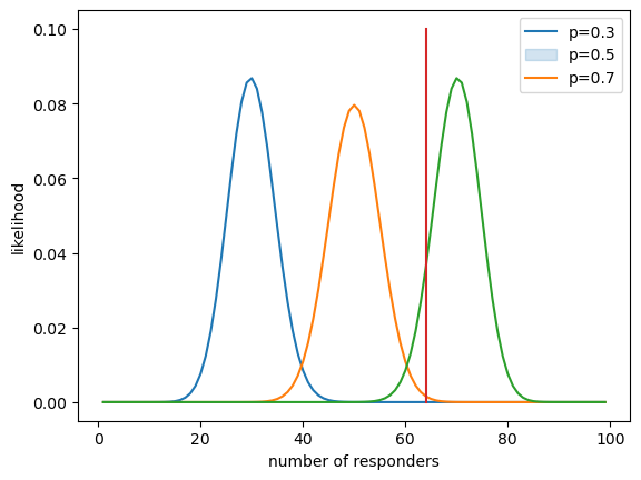
Figure 11.3

likeDf['uniform_prior'] = 1 / likeDf.shape[0]

marginal_likelihood = np.sum(binom.pmf(nResponders, nTested, likeDf.presp) * likeDf.uniform_prior)

bayesDf = pd.DataFrame({'steps': np.arange(.01, 1.0, .01)})
bayesDf['likelihoods'] = binom.pmf(nResponders, nTested, bayesDf.steps)
bayesDf['priors'] = 1 / bayesDf.shape[0]
bayesDf['posteriors'] = (bayesDf.likelihoods * bayesDf.priors) / marginal_likelihood
maxidx = bayesDf.posteriors.argmax()
MAP = bayesDf.steps[maxidx]

sns.lineplot(data=bayesDf, x='steps', y='posteriors')
plt.scatter([MAP], bayesDf.posteriors.max(), color='black')
sns.lineplot(data=bayesDf, x='steps', y='priors', color='black', linewidth=.5, linestyle='dashed')
plt.xlabel('p(respond)')
plt.ylabel('posterior probability of the observed data')

Text(0, 0.5, 'posterior probability of the observed data')

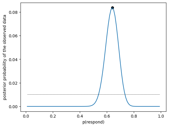
Figure 11.4

fig, ax = plt.subplots(2, 2, figsize=(12,8))


bayesDf = pd.DataFrame({'steps': np.arange(.01, 1.0, .01)})
bayesDf['likelihoods'] = binom.pmf(nResponders, nTested, bayesDf.steps)
bayesDf['priors_flat'] = 1 / bayesDf.shape[0]
bayesDf['priors_absolute'] = 0
bayesDf.loc[bayesDf.steps > 0.8, 'priors_absolute'] = 1
bayesDf.priors_absolute = bayesDf.priors_absolute / bayesDf.priors_absolute.sum()
bayesDf['priors_empirical_weak'] = binom.pmf(10, 20, bayesDf.steps) / np.sum(binom.pmf(10, 20, bayesDf.steps))
bayesDf['priors_empirical_strong'] = binom.pmf(250, 500, bayesDf.steps) / np.sum(binom.pmf(250, 500, bayesDf.steps))

marginal_likelihood_flat = np.sum(binom.pmf(nResponders, nTested, bayesDf.steps) * bayesDf.priors_flat)
marginal_likelihood_weak = np.sum(binom.pmf(nResponders, nTested, bayesDf.steps) * bayesDf.priors_empirical_weak)
marginal_likelihood_strong = np.sum(binom.pmf(nResponders, nTested, bayesDf.steps) * bayesDf.priors_empirical_strong)
marginal_likelihood_absolute = np.sum(binom.pmf(nResponders, nTested, bayesDf.steps) * bayesDf.priors_absolute)


bayesDf['posteriors_flat'] = (bayesDf.likelihoods * bayesDf.priors_flat) / marginal_likelihood_flat
bayesDf['posteriors_weak'] = (bayesDf.likelihoods * bayesDf.priors_empirical_weak) / marginal_likelihood_weak
bayesDf['posteriors_strong'] = (bayesDf.likelihoods * bayesDf.priors_empirical_strong) / marginal_likelihood_strong
bayesDf['posteriors_absolute'] = (bayesDf.likelihoods * bayesDf.priors_absolute) / marginal_likelihood_absolute

sns.lineplot(data=bayesDf, x='steps', y='posteriors_flat', ax=ax[0][0], color='blue')
sns.lineplot(data=bayesDf, x='steps', y='posteriors_weak', ax=ax[0][0], color='red')
sns.lineplot(data=bayesDf, x='steps', y='priors_empirical_weak', ax=ax[0][0], linestyle='dotted')

sns.lineplot(data=bayesDf, x='steps', y='posteriors_weak', ax=ax[0][1], color='blue')
sns.lineplot(data=bayesDf, x='steps', y='posteriors_strong', ax=ax[0][1], color='red')
sns.lineplot(data=bayesDf, x='steps', y='priors_empirical_strong', ax=ax[0][1], linestyle='dotted')

sns.lineplot(data=bayesDf, x='steps', y='posteriors_absolute', ax=ax[1][0], color='blue')
bayesDf.loc[bayesDf.steps > 0.8, 'priors_absolute'] = 0.7  # rescale for figure
sns.lineplot(data=bayesDf, x='steps', y='priors_absolute', ax=ax[1][0], linestyle='dotted')


for i in range(2):
    for j in range(2):
        ax[i][j].set_xlabel("p(heads)")
        ax[i][j].set_ylabel("Posterior probability")

ax[1][1].set_visible(False)

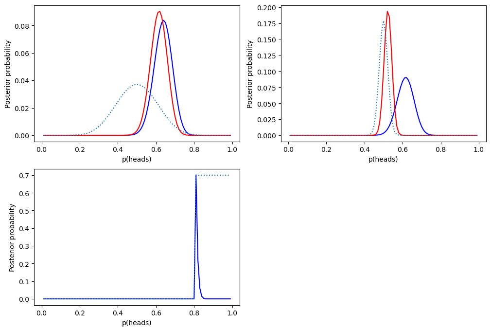
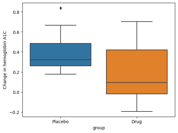
Figure 11.5

nsubs = 40
effect_size = 0.2
rng = np.random.default_rng(12345)

drugDf = pd.DataFrame({'group': ['Drug' if rng.uniform() > .5 else 'Placebo' for i in range(nsubs)]})
drugDf['hbchange'] =  rng.uniform(size=nsubs) - (drugDf.group == 'Drug') * effect_size

sns.boxplot(data=drugDf, x='group', y='hbchange')
plt.ylabel('Change in hemoglobin A1C')

Text(0, 0.5, 'Change in hemoglobin A1C')

T-test for drug example

tt = pg.ttest(x=drugDf.query('group == "Placebo"').hbchange, 
              y=drugDf.query('group == "Drug"').hbchange,
              correction=True, alternative='greater')
tt

	T	dof	alternative	p-val	CI95%	cohen-d	BF10	power
T-test	2.60501	31.58191	greater	0.006945	[0.07, inf]	0.823776	8.104	0.819463

Bayes factor for drug example

BF10 is generated by pg.ttest in cell above, but its method for one vs. two-tailed tests differs from that used in the BayesFactor package in R.

%%R -i drugDf

library(BayesFactor)
bf_drug <- ttestBF(
  formula = hbchange ~ group, data = drugDf,
  nullInterval = c(0, Inf)
)
bf_drug

R[write to console]: Loading required package: coda

R[write to console]: Loading required package: Matrix

R[write to console]: ************
Welcome to BayesFactor 0.9.12-4.4. If you have questions, please contact Richard Morey (richarddmorey@gmail.com).

Type BFManual() to open the manual.
************

Bayes factor analysis
--------------

[1] Alt., r=0.707 0<d<Inf   

 : 

0.1007666

 ±

0

%

[2] Alt., r=0.707 !(0<d<Inf)

 : 

8.00271  

 ±

0

%

Against denominator:

Null, mu1-mu2 = 0

---
Bayes factor type: 

BFindepSample

, 

JZS

Bayes factor for one-sided tests

%%R 

bf_drug[1]/bf_drug[2]

Bayes factor analysis
--------------

[1] Alt., r=0.707 0<d<Inf

 : 

0.01259155

 ±

0

%

Against denominator:

Alternative, r = 0.707106781186548, mu =/= 0 !(0<d<Inf)

---
Bayes factor type: 

BFindepSample

, 

JZS

Table 11.1

# Compute credible intervals for example

nsamples = 100000

# create random uniform variates for x and y
x = rng.uniform(size=nsamples)
y = rng.uniform(size=nsamples)

# create f(x)
fx = binom.pmf(nResponders,nTested, x)

# accept samples where y < f(x)
accepted_samples = x[y < fx]

credible_interval = scoreatpercentile(accepted_samples, (2.5, 97.5))

credible_interval

array([0.54525307, 0.72923171])

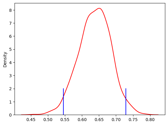
Figure 11.6

sns.kdeplot(accepted_samples, color='red')
for c in credible_interval:
    plt.plot([c, c], [0, 2], color='blue')