Chapter 12: Modeling categorical relationships

import pandas as pd
import sidetable
import numpy as np
import matplotlib.pyplot as plt
import seaborn as sns
from scipy.stats import norm, t, binom, chi2
import pingouin as pg
import matplotlib

import rpy2.robjects as ro
from rpy2.robjects.packages import importr
from rpy2.robjects import pandas2ri
pandas2ri.activate()
from rpy2.robjects.conversion import localconverter
%load_ext rpy2.ipython

# import NHANES package
base = importr('NHANES')

with localconverter(ro.default_converter + pandas2ri.converter):
  NHANES = ro.conversion.rpy2py(ro.r['NHANES'])

 
NHANES = NHANES.drop_duplicates(subset='ID')
NHANES_adult = NHANES.dropna(subset=['Weight']).query('Age > 17 and BPSysAve > 0')

rng = np.random.default_rng(123456)

Table 12.1

candyDf = pd.DataFrame({'Candy Type': ["chocolate", "licorice", "gumball"],
                            'Count': [30, 33, 37]})
candyDf['nullExpectation'] = [candyDf.Count.sum() / 3] * 3
candyDf['squaredDifference'] = (candyDf.Count - candyDf.nullExpectation) ** 2

candyDf

	Candy Type	Count	nullExpectation	squaredDifference
0	chocolate	30	33.333333	11.111111
1	licorice	33	33.333333	0.111111
2	gumball	37	33.333333	13.444444

Figure 12.1

chisqVal = np.sum(candyDf.squaredDifference / candyDf.nullExpectation)
chisqVal

0.7399999999999999

x = np.arange(0.01, 20, .01)
dfvals = [1, 2, 4, 8]

x_df = [(i, j) for i in x for j in dfvals]

chisqDf = pd.DataFrame(x_df, columns = ['x', 'df'])
chisqDf['chisq'] = chi2.pdf(chisqDf.x, chisqDf.df)
for df in dfvals:
    chisqDf.loc[chisqDf.df == df, 'chisq'] = chisqDf[chisqDf.df == df]['chisq'] / chisqDf[chisqDf.df == df]['chisq'].max()
fig, ax = plt.subplots(1, 2, figsize=(12,6))

sns.lineplot(data=chisqDf, x='x', y='chisq', style='df', ax=ax[0])
ax[0].set_xlabel("Chi-squared values")
ax[0].set_ylabel('Density')


# simulate 50,000 sums of 8 standard normal random variables and compare
# to theoretical chi-squared distribution

# create a matrix with 50k columns of 8 rows of squared normal random variables
dSum = (rng.normal(size=(50000, 8)) ** 2).sum(axis=1)

sns.histplot(dSum, ax=ax[1], stat='density')
ax[1].set_ylabel("Density")
ax[1].set_xlabel("Sum of squared random normal variables")

csDf = pd.DataFrame({'x': np.arange(0.01, 30, 0.01)})
csDf['chisq'] = chi2.pdf(csDf.x, 8)
_ =sns.lineplot(data=csDf, x='x', y='chisq', ax=ax[1], color='black')

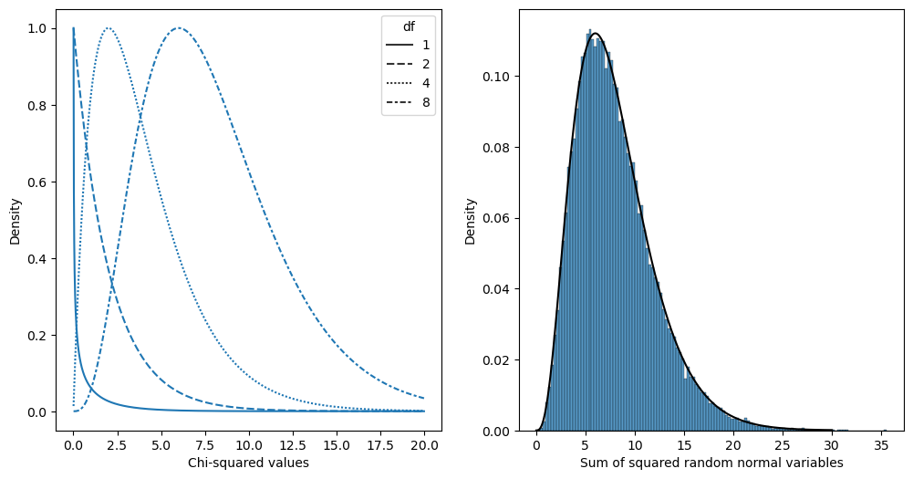
Table 12.2

stopData = pd.read_csv('https://raw.githubusercontent.com/statsthinking21/statsthinking21-figures-data/main/CT_data_cleaned.csv')
table = pd.crosstab(stopData['driver_race'], stopData['search_conducted'], margins=True)
print(table)
n = stopData.shape[0]
print('')
print('Normalized:')
table_normalized = pd.crosstab(stopData['driver_race'], stopData['search_conducted'], margins=True, normalize='all')
print(table_normalized)

search_conducted   False  True     All
driver_race                           
Black              36244  1219   37463
White             239241  3108  242349
All               275485  4327  279812

Normalized:
search_conducted     False      True       All
driver_race                                   
Black             0.129530  0.004356  0.133886
White             0.855006  0.011107  0.866114
All               0.984536  0.015464  1.000000

Chi-squared test result

expected = np.outer(table_normalized.values[:2, 2], table_normalized.values[2, :2]) * n
actual = pd.crosstab(stopData['driver_race'], stopData['search_conducted'], margins=False)
diff = expected - actual
stdSqDiff = diff **2 / expected
chisq = stdSqDiff.sum().sum()
pval = chi2.pdf(chisq, 1)
pval

1.9001204194035138e-182

_, _, stats = pg.chi2_independence(stopData, 'driver_race', 'search_conducted')
stats[stats.test=='pearson']

	test	lambda	chi2	dof	pval	cramer	power
0	pearson	1.0	827.005515	1.0	7.255988e-182	0.054365	1.0

Table 12.3

summaryDfResids = diff/ np.sqrt(expected)
summaryDfResids

search_conducted	False	True
driver_race
Black	3.330746	-26.576456
White	-1.309550	10.449072

Bayes factor

%%R -i actual

# compute Bayes factor
# using independent multinomial sampling plan in which row totals (driver race)
# are fixed
library(BayesFactor)
bf <-
  contingencyTableBF(as.matrix(actual),
  sampleType = "indepMulti",
  fixedMargin = "cols"
)
bf

R[write to console]: Loading required package: coda

R[write to console]: Loading required package: Matrix

R[write to console]: ************
Welcome to BayesFactor 0.9.12-4.4. If you have questions, please contact Richard Morey (richarddmorey@gmail.com).

Type BFManual() to open the manual.
************

Bayes factor analysis
--------------

[1] Non-indep. (a=1)

 : 

1.753219e+142

 ±

0

%

Against denominator:

Null, independence, a = 1

---
Bayes factor type: 

BFcontingencyTable

, 

independent multinomial

Table 12.4

NHANES_sleep = NHANES.query('Age > 17').dropna(subset=['SleepTrouble', 'Depressed'])
depressedSleepTrouble = pd.crosstab( NHANES_sleep.Depressed, NHANES_sleep.SleepTrouble)
depressedSleepTrouble

SleepTrouble	No	Yes
Depressed
None	2631	678
Several	423	254
Most	140	146

Chi-squared result

_, _, stats = pg.chi2_independence(NHANES_sleep, 'SleepTrouble', 'Depressed')
stats[stats.test=='pearson']

	test	lambda	chi2	dof	pval	cramer	power
0	pearson	1.0	194.653393	2.0	5.389552e-43	0.213459	1.0

Bayes factor

%%R -i depressedSleepTrouble

# compute bayes factor, using a joint multinomial sampling plan
bf <-
  contingencyTableBF(
    as.matrix(depressedSleepTrouble),
    sampleType = "jointMulti"
  )
bf

Bayes factor analysis
--------------

[1] Non-indep. (a=1)

 : 

8.541445e+35

 ±

0

%

Against denominator:

Null, independence, a = 1

---
Bayes factor type: 

BFcontingencyTable

, 

joint multinomial