Chapter 17: Practical statistical modeling
Contents
Chapter 17: Practical statistical modeling#
Note: The results may differ slightly between Python and R implementations, due to difference in random seeds as well as slight differences in data filtering between the two notebooks.
import pandas as pd
import numpy as np
import matplotlib.pyplot as plt
import seaborn as sns
from scipy.stats import norm, t, binom, scoreatpercentile, pearsonr, chi2
from scipy.spatial.distance import cdist
import pingouin as pg
import matplotlib
import statsmodels.api as sm
import statsmodels.formula.api as smf
from sklearn.metrics import r2_score, mean_squared_error
from sklearn.model_selection import KFold
from sklearn.preprocessing import scale
from sklearn.cluster import KMeans, AgglomerativeClustering
from sklearn.metrics import adjusted_rand_score
from scipy.cluster import hierarchy
from scipy.special import logit
from sklearn.decomposition import PCA
import yellowbrick as yb
from statsmodels.genmod.bayes_mixed_glm import BinomialBayesMixedGLM

%matplotlib inline
import rpy2.robjects as ro
from rpy2.robjects.packages import importr
from rpy2.robjects import pandas2ri
pandas2ri.activate()

base = importr('lme4')
base = importr('tidyverse')
base = importr('broom')

%load_ext rpy2.ipython

rng = np.random.default_rng(1234567)
Figure 17.1 Outliers and influential observations#
npts = 24
outlier_df = pd.DataFrame({'Y': rng.normal(size=npts)})
outlier_df['X'] = outlier_df.Y * 0.4 + rng.normal(size=npts)

def get_cooksD(X, Y):
    X = sm.add_constant(X)
    model = sm.OLS(Y, X).fit()
    influence = model.get_influence()
    return(influence.cooks_distance[0])

#sns.set_context("talk", font_scale=1.2)
plt.figure(figsize=(8,8))
g = sns.JointGrid(data=outlier_df,
                  x="X",
                  y="Y")
g.plot_joint(sns.regplot, ci=None, scatter_kws={'s': 20 + get_cooksD(outlier_df.X, outlier_df.Y)*500})
g.plot_marginals(sns.boxplot)
<seaborn.axisgrid.JointGrid at 0x7f308864fd90>
<Figure size 800x800 with 0 Axes>
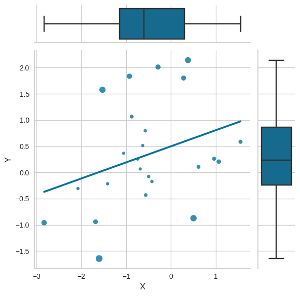
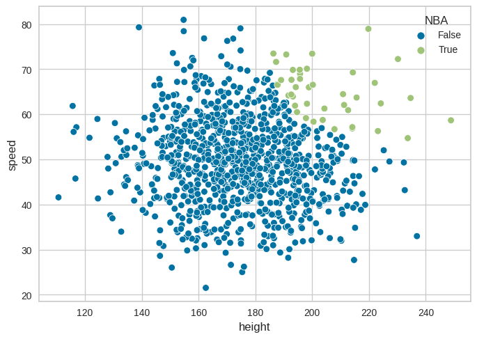
Figure 17.2: Collider bias#
# https://observablehq.com/@herbps10/collider-bias
npts = 1000

conf_df = pd.DataFrame({'height': rng.normal(175, 20, npts),
                        'speed': rng.normal(50, 10, npts)})
conf_df['zheight'] = scale(conf_df.height)
conf_df['zspeed'] = scale(conf_df.speed)
conf_df['speedXheight'] = conf_df.zheight * conf_df.zspeed
conf_df['NBA'] = (conf_df.speedXheight > scoreatpercentile(conf_df.speedXheight, 90)) & \
    (conf_df.speed > conf_df.speed.mean()) & (conf_df.height > conf_df.height.mean())

sns.scatterplot(data=conf_df, x='height', y='speed', hue='NBA')
<Axes: xlabel='height', ylabel='speed'>
print(smf.ols(formula='speed ~ 1 + height', data=conf_df).fit().summary())
                            OLS Regression Results
==============================================================================
Dep. Variable:                  speed   R-squared:                       0.001
Model:                            OLS   Adj. R-squared:                  0.000
Method:                 Least Squares   F-statistic:                     1.122
Date:                Tue, 21 Feb 2023   Prob (F-statistic):              0.290
Time:                        21:53:20   Log-Likelihood:                -3693.9
No. Observations:                1000   AIC:                             7392.
Df Residuals:                     998   BIC:                             7402.
Df Model:                           1
Covariance Type:            nonrobust
==============================================================================
                 coef    std err          t      P>|t|      [0.025      0.975]
------------------------------------------------------------------------------
Intercept     52.8286      2.667     19.811      0.000      47.596      58.062
height        -0.0160      0.015     -1.059      0.290      -0.046       0.014
==============================================================================
Omnibus:                        6.119   Durbin-Watson:                   1.994
Prob(Omnibus):                  0.047   Jarque-Bera (JB):                6.187
Skew:                           0.191   Prob(JB):                       0.0453
Kurtosis:                       2.954   Cond. No.                     1.53e+03
==============================================================================

Notes:
[1] Standard Errors assume that the covariance matrix of the errors is correctly specified.
[2] The condition number is large, 1.53e+03. This might indicate that there are
strong multicollinearity or other numerical problems.
Model with NBA player status (collider)
print(smf.ols(formula='speed ~ 1 + height + NBA', data=conf_df).fit().summary())
                            OLS Regression Results
==============================================================================
Dep. Variable:                  speed   R-squared:                       0.121
Model:                            OLS   Adj. R-squared:                  0.119
Method:                 Least Squares   F-statistic:                     68.71
Date:                Tue, 21 Feb 2023   Prob (F-statistic):           1.11e-28
Time:                        21:53:20   Log-Likelihood:                -3629.9
No. Observations:                1000   AIC:                             7266.
Df Residuals:                     997   BIC:                             7281.
Df Model:                           2
Covariance Type:            nonrobust
===============================================================================
                  coef    std err          t      P>|t|      [0.025      0.975]
-------------------------------------------------------------------------------
Intercept      61.3954      2.608     23.541      0.000      56.277      66.513
NBA[T.True]    17.6543      1.513     11.668      0.000      14.685      20.623
height         -0.0692      0.015     -4.640      0.000      -0.098      -0.040
==============================================================================
Omnibus:                        3.634   Durbin-Watson:                   1.988
Prob(Omnibus):                  0.163   Jarque-Bera (JB):                3.491
Skew:                           0.127   Prob(JB):                        0.175
Kurtosis:                       3.137   Cond. No.                     1.62e+03
==============================================================================

Notes:
[1] Standard Errors assume that the covariance matrix of the errors is correctly specified.
[2] The condition number is large, 1.62e+03. This might indicate that there are
strong multicollinearity or other numerical problems.
same regression only on the NBA players, where we see a strong negative relationship between speed and height:
print(smf.ols(formula='speed ~ 1 + height', data=conf_df.query('NBA == True')).fit().summary())
                            OLS Regression Results
==============================================================================
Dep. Variable:                  speed   R-squared:                       0.116
Model:                            OLS   Adj. R-squared:                  0.094
Method:                 Least Squares   F-statistic:                     5.261
Date:                Tue, 21 Feb 2023   Prob (F-statistic):             0.0271
Time:                        21:53:20   Log-Likelihood:                -128.55
No. Observations:                  42   AIC:                             261.1
Df Residuals:                      40   BIC:                             264.6
Df Model:                           1
Covariance Type:            nonrobust
==============================================================================
                 coef    std err          t      P>|t|      [0.025      0.975]
------------------------------------------------------------------------------
Intercept     90.6515     11.265      8.047      0.000      67.885     113.418
height        -0.1258      0.055     -2.294      0.027      -0.237      -0.015
==============================================================================
Omnibus:                        4.981   Durbin-Watson:                   2.303
Prob(Omnibus):                  0.083   Jarque-Bera (JB):                3.737
Skew:                           0.678   Prob(JB):                        0.154
Kurtosis:                       3.544   Cond. No.                     2.83e+03
==============================================================================

Notes:
[1] Standard Errors assume that the covariance matrix of the errors is correctly specified.
[2] The condition number is large, 2.83e+03. This might indicate that there are
strong multicollinearity or other numerical problems.
Example 1: Self-regulation and arrest#
behavdata = pd.read_csv('https://raw.githubusercontent.com/statsthinking21/statsthinking21-figures-data/main/Eisenberg/meaningful_variables.csv')
behavdata.set_index('subcode', inplace=True)
demoghealthdata = pd.read_csv('https://raw.githubusercontent.com/statsthinking21/statsthinking21-figures-data/main/Eisenberg/demographic_health.csv')
demoghealthdata.set_index('subcode', inplace=True)
sexdict = {1:'Female', 0:'Male'}
demoghealthdata['Sex'] = [sexdict[i] for i in demoghealthdata['Sex']]
alldata = demoghealthdata.join(behavdata, how='inner')

rename_dict = {
    'upps_impulsivity_survey': 'UPPS',
    'sensation_seeking_survey': 'SSS',
    'dickman_survey': 'Dickman',
    'bis11_survey': 'BIS11'
}

impulsivity_vars = []
for column in alldata.columns:
    for k, v in rename_dict.items():
        if k in column:
            alldata.rename(columns={column: column.replace(k, v)}, inplace=True)
            impulsivity_vars.append(column.replace(k, v))
Table 17.1#
Frequency distribution of number of reported arrests in the Eisenberg et al. dataset
arrestdata = alldata.dropna(subset=['ArrestedChargedLifeCount'])
arrestdata.loc['everArrested'] = arrestdata.ArrestedChargedLifeCount > 0

pd.DataFrame({
    'number': arrestdata.ArrestedChargedLifeCount.value_counts(),
    'proportion': arrestdata.ArrestedChargedLifeCount.value_counts()/arrestdata.shape[0]})
| number | proportion | |
|---|---|---|
| 0.0 | 409 | 0.783525 |
| 1.0 | 58 | 0.111111 |
| 2.0 | 33 | 0.063218 |
| 3.0 | 9 | 0.017241 |
| 5.0 | 5 | 0.009579 |
| 4.0 | 5 | 0.009579 |
| 6.0 | 2 | 0.003831 |
Figure 17.3#
impulsivity_data = alldata.dropna(subset=['ArrestedChargedLifeCount',
           'TrafficTicketsLastYearCount',
           'TrafficAccidentsLifeCount', 'Age','Sex'])
impulsivity_data['everArrested'] = impulsivity_data.ArrestedChargedLifeCount > 0
cc = impulsivity_data[impulsivity_vars].corr()

sns.clustermap(cc, method='average', annot=True)
/tmp/ipykernel_2300/2323405881.py:4: SettingWithCopyWarning:
A value is trying to be set on a copy of a slice from a DataFrame.
Try using .loc[row_indexer,col_indexer] = value instead

See the caveats in the documentation: https://pandas.pydata.org/pandas-docs/stable/user_guide/indexing.html#returning-a-view-versus-a-copy
  impulsivity_data['everArrested'] = impulsivity_data.ArrestedChargedLifeCount > 0
<seaborn.matrix.ClusterGrid at 0x7f3143067dc0>
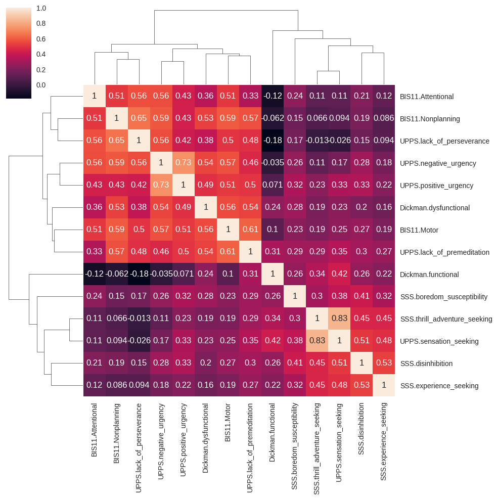
Figure 17.4#
cls = AgglomerativeClustering(n_clusters=2)
cls.fit(cc)
# 0 is sensation seeking, 1 is impulsivity
varnames = ['mean_senseek', 'mean_impulsivity']
newvars = {}

for cluster in range(2):
    vars = [impulsivity_vars[i] for i in range(len(impulsivity_vars)) if cls.labels_[i] == cluster]
    newvars[varnames[cluster]] = impulsivity_data.loc[:, vars].mean(axis=1, skipna=True)

for k, v, in newvars.items():
    impulsivity_data[k] = scale(v)


g = sns.PairGrid(impulsivity_data[varnames])

def corrfunc(x, y, hue=None, ax=None, **kws):
    """Plot the correlation coefficient in the top left hand corner of a plot."""
    r, _ = pearsonr(x, y)
    ax = ax or plt.gca()
    ax.annotate(f'r = {r:.2f}', xy=(.2, .5), size=24, xycoords=ax.transAxes)

g.map_upper(corrfunc)
g.map_lower(sns.regplot, color='black')
g.map_diag(sns.histplot, kde=True, legend=False)
plt.show()
/tmp/ipykernel_2300/221161768.py:12: SettingWithCopyWarning:
A value is trying to be set on a copy of a slice from a DataFrame.
Try using .loc[row_indexer,col_indexer] = value instead

See the caveats in the documentation: https://pandas.pydata.org/pandas-docs/stable/user_guide/indexing.html#returning-a-view-versus-a-copy
  impulsivity_data[k] = scale(v)
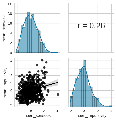
Figure 17.5#
fig, ax = plt.subplots(1, 2, figsize=(12,6))

sns.boxplot(data=impulsivity_data, x='everArrested', y='mean_impulsivity', ax=ax[0])
sns.swarmplot(data=impulsivity_data, x='everArrested', y='mean_impulsivity', ax=ax[0], color='black', alpha=0.5)

sns.boxplot(data=impulsivity_data, x='everArrested', y='mean_senseek', ax=ax[1])
sns.swarmplot(data=impulsivity_data, x='everArrested', y='mean_senseek', ax=ax[1], color='black', alpha=0.5)
<Axes: xlabel='everArrested', ylabel='mean_senseek'>
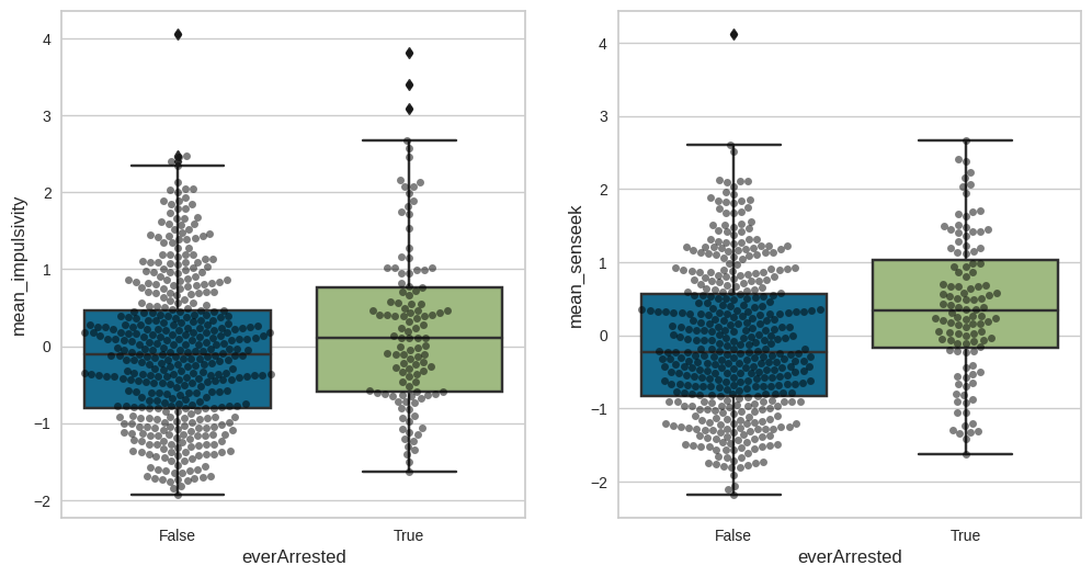
t-test output for the mean impulsivity scores:
tt = pg.ttest(x=impulsivity_data.query('everArrested == True').mean_impulsivity,
              y=impulsivity_data.query('everArrested == False').mean_impulsivity,
              alternative='greater')
tt
| T | dof | alternative | p-val | CI95% | cohen-d | BF10 | power | |
|---|---|---|---|---|---|---|---|---|
| T-test | 2.910521 | 160.928447 | greater | 0.00206 | [0.14, inf] | 0.334129 | 13.485 | 0.931108 |
t-test output for the sensation seeking variable:
tt = pg.ttest(x=impulsivity_data.query('everArrested == True').mean_senseek,
              y=impulsivity_data.query('everArrested == False').mean_senseek,
              alternative='greater')
tt
| T | dof | alternative | p-val | CI95% | cohen-d | BF10 | power | |
|---|---|---|---|---|---|---|---|---|
| T-test | 4.769141 | 182.383008 | greater | 0.000002 | [0.32, inf] | 0.496897 | 1.11e+04 | 0.998687 |
Figure 17.6: Logistic regression#
rng = np.random.default_rng(1234567)
n = 100
b0 = 100
b1 = 5

logreg_df = pd.DataFrame({'x': rng.normal(0, 10, n)})
logreg_df['y'] = b0 + b1 * logreg_df.x + rng.normal(0, 3, n)
logreg_df['y_bin'] =  (rng.uniform(size=n) < 1  /(1 + np.exp( -(logreg_df.y - logreg_df.y.mean()) / logreg_df.y.std()))).astype('int')
logreg_df['y_bin_jitter'] =  logreg_df.y_bin +  rng.uniform(-.01, .01, size=n)


lm = smf.ols(formula='y_bin ~ 1 + x', data=logreg_df)
lm_result = lm.fit()
logreg_df['lm_pred'] = lm_result.predict()

logistic = smf.logit(formula='y_bin ~ 1 + x', data=logreg_df)
logistic_result = logistic.fit()
logreg_df['logistic_pred'] = logistic_result.predict()


fig, ax = plt.subplots(1, 2, figsize=(12,6))

sns.scatterplot(data=logreg_df, x='x', y='y_bin_jitter', ax=ax[0])
sns.lineplot(data=logreg_df, x='x', y='lm_pred', ax=ax[0])
ax[0].set_title('A: Linear regression')

sns.scatterplot(data=logreg_df, x='x', y='y_bin_jitter', ax=ax[1])
sns.lineplot(data=logreg_df, x='x', y='logistic_pred', ax=ax[1])
ax[0].set_title('A: Logistic regression')
Optimization terminated successfully.
         Current function value: 0.533560
         Iterations 6
Text(0.5, 1.0, 'A: Logistic regression')
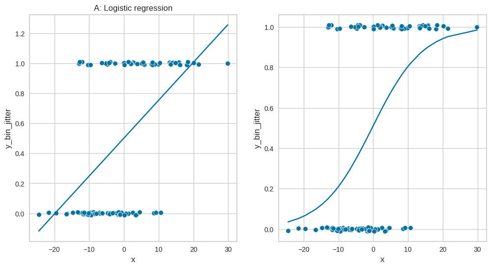
Logistic regression output:
print(logistic_result.summary())
                           Logit Regression Results
==============================================================================
Dep. Variable:                  y_bin   No. Observations:                  100
Model:                          Logit   Df Residuals:                       98
Method:                           MLE   Df Model:                            1
Date:                Tue, 21 Feb 2023   Pseudo R-squ.:                  0.2300
Time:                        21:53:26   Log-Likelihood:                -53.356
converged:                       True   LL-Null:                       -69.295
Covariance Type:            nonrobust   LLR p-value:                 1.642e-08
==============================================================================
                 coef    std err          z      P>|z|      [0.025      0.975]
------------------------------------------------------------------------------
Intercept      0.0447      0.238      0.188      0.851      -0.422       0.512
x              0.1369      0.030      4.604      0.000       0.079       0.195
==============================================================================
Logistic regression output for impulsivity dataset
impulsivity_data.loc[:, 'AgeSquared'] = (impulsivity_data.Age - impulsivity_data.Age.mean()) ** 2
impulsivity_data.loc[:, 'everArrestedInt'] = impulsivity_data.everArrested.astype('int')

# the following is for R
impulsivity_data.loc[:, 'SexInt'] = [1 if i == 'Male' else 0 for i in impulsivity_data.Sex]
impulsivity_data = impulsivity_data[['everArrestedInt', 'mean_impulsivity', 'mean_senseek', 'Age', 'AgeSquared', 'Sex', 'SexInt']]

glm_imp_arrest = smf.glm(
    formula='everArrestedInt ~ 1 + mean_impulsivity + mean_senseek + Age +   Sex',
    data=impulsivity_data,
    family=sm.families.Binomial())
logistic_result = glm_imp_arrest.fit()

print(logistic_result.summary())
                 Generalized Linear Model Regression Results
==============================================================================
Dep. Variable:        everArrestedInt   No. Observations:                  521
Model:                            GLM   Df Residuals:                      516
Model Family:                Binomial   Df Model:                            4
Link Function:                  Logit   Scale:                          1.0000
Method:                          IRLS   Log-Likelihood:                -250.58
Date:                Tue, 21 Feb 2023   Deviance:                       501.15
Time:                        21:53:26   Pearson chi2:                     532.
No. Iterations:                     5   Pseudo R-squ. (CS):            0.07599
Covariance Type:            nonrobust
====================================================================================
                       coef    std err          z      P>|z|      [0.025      0.975]
------------------------------------------------------------------------------------
Intercept           -3.3826      0.558     -6.066      0.000      -4.476      -2.290
Sex[T.Male]          0.6510      0.238      2.736      0.006       0.185       1.117
mean_impulsivity     0.2859      0.113      2.528      0.011       0.064       0.508
mean_senseek         0.3778      0.118      3.214      0.001       0.147       0.608
Age                  0.0485      0.014      3.372      0.001       0.020       0.077
====================================================================================
/tmp/ipykernel_2300/1360466332.py:1: SettingWithCopyWarning:
A value is trying to be set on a copy of a slice from a DataFrame.
Try using .loc[row_indexer,col_indexer] = value instead

See the caveats in the documentation: https://pandas.pydata.org/pandas-docs/stable/user_guide/indexing.html#returning-a-view-versus-a-copy
  impulsivity_data.loc[:, 'AgeSquared'] = (impulsivity_data.Age - impulsivity_data.Age.mean()) ** 2
/tmp/ipykernel_2300/1360466332.py:2: SettingWithCopyWarning:
A value is trying to be set on a copy of a slice from a DataFrame.
Try using .loc[row_indexer,col_indexer] = value instead

See the caveats in the documentation: https://pandas.pydata.org/pandas-docs/stable/user_guide/indexing.html#returning-a-view-versus-a-copy
  impulsivity_data.loc[:, 'everArrestedInt'] = impulsivity_data.everArrested.astype('int')
/tmp/ipykernel_2300/1360466332.py:5: SettingWithCopyWarning:
A value is trying to be set on a copy of a slice from a DataFrame.
Try using .loc[row_indexer,col_indexer] = value instead

See the caveats in the documentation: https://pandas.pydata.org/pandas-docs/stable/user_guide/indexing.html#returning-a-view-versus-a-copy
  impulsivity_data.loc[:, 'SexInt'] = [1 if i == 'Male' else 0 for i in impulsivity_data.Sex]
Compare with R results
%%R -i impulsivity_data

glm_imp_arrest = glm('everArrestedInt ~ 1 + mean_impulsivity + mean_senseek + Age +  SexInt',
    data=impulsivity_data,
    family='binomial')

print(summary(glm_imp_arrest))
Call:
glm(formula = "everArrestedInt ~ 1 + mean_impulsivity + mean_senseek + Age +  SexInt",
    family = "binomial", data = impulsivity_data)
Deviance Residuals:
Min
1Q
Median
3Q
Max
-1.3386
-0.7119
-0.5722
-0.3575
2.4726
Coefficients:
Estimate
Std. Error
z value
Pr(>|z|)
(Intercept)
-3.38260
0.55767
-6.066
1.31e-09
***
mean_impulsivity
0.28595
0.11309
2.528
0.011459
*
mean_senseek
0.37779
0.11754
3.214
0.001308
**
Age
0.04849
0.01438
3.372
0.000746
***
SexInt
0.65095
0.23793
2.736
0.006222
**
---
Signif. codes:
0 ‘***’ 0.001 ‘**’ 0.01 ‘*’ 0.05 ‘.’ 0.1 ‘ ’ 1
(Dispersion parameter for
binomial
family taken to be
1
)
Null deviance: 542.33 on 520 degrees of freedom
Residual deviance: 501.15 on 516 degrees of freedom
AIC:
511.15
Number of Fisher Scoring iterations:
4
Test for overdispersion#
There is no built-in test for overdispersion in Python. However, we can perform a simple chi-squared test for overdispersion, by dividing the Pearson chi-squared statistic by the residual degrees of freedom, which gives the same result as the R overdispersion test using the chi-squared.
chisq_stat = logistic_result.pearson_chi2 / logistic_result.df_resid
print('dispersion = ', chisq_stat)

pval = 1 - chi2.cdf(logistic_result.pearson_chi2, logistic_result.df_resid)
print('pvalue (alternative ="greater") = ', pval)
dispersion =  1.0305993193299552
pvalue (alternative ="greater") =  0.3059811971051235
Compare to R result
%%R

library('DHARMa')

print(testDispersion(glm_imp_arrest, alternative='greater', type='PearsonChisq'))
R[write to console]: This is DHARMa 0.4.6. For overview type '?DHARMa'. For recent changes, type news(package = 'DHARMa')
Parametric dispersion test via mean Pearson-chisq statistic
data:
glm_imp_arrest
dispersion = 1.0306, df = 516, p-value = 0.306
alternative hypothesis:
greater
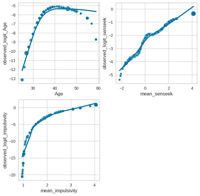
Figure 17.7#
# the statsmodels lowess smoother returned all zeros, so we are using this
# from https://xavierbourretsicotte.github.io/loess.html

from math import ceil
import numpy as np
from scipy import linalg

def lowess_ag(x, y, f=2. / 3., iter=3):
    """lowess(x, y, f=2./3., iter=3) -> yest
    Lowess smoother: Robust locally weighted regression.
    The lowess function fits a nonparametric regression curve to a scatterplot.
    The arrays x and y contain an equal number of elements; each pair
    (x[i], y[i]) defines a data point in the scatterplot. The function returns
    the estimated (smooth) values of y.
    The smoothing span is given by f. A larger value for f will result in a
    smoother curve. The number of robustifying iterations is given by iter. The
    function will run faster with a smaller number of iterations.
    """
    n = len(x)
    r = int(ceil(f * n))
    h = [np.sort(np.abs(x - x[i]))[r] for i in range(n)]
    w = np.clip(np.abs((x[:, None] - x[None, :]) / h), 0.0, 1.0)
    w = (1 - w ** 3) ** 3
    yest = np.zeros(n)
    delta = np.ones(n)
    for iteration in range(iter):
        for i in range(n):
            weights = delta * w[:, i]
            b = np.array([np.sum(weights * y), np.sum(weights * y * x)])
            A = np.array([[np.sum(weights), np.sum(weights * x)],
                          [np.sum(weights * x), np.sum(weights * x * x)]])
            beta = linalg.solve(A, b)
            yest[i] = beta[0] + beta[1] * x[i]

        residuals = y - yest
        s = np.median(np.abs(residuals))
        delta = np.clip(residuals / (6.0 * s), -1, 1)
        delta = (1 - delta ** 2) ** 2

    return yest
def cat_logit_est(iv, df, max_bins=18):
    ncats = np.min((max_bins, np.round(iv.unique().shape[0] / 2).astype('int')))
    iv_cut = pd.cut(iv, ncats)
    glm_imp_arrest = smf.glm(
        formula='everArrestedInt ~ 1 + iv_cut', data=df,
        family=sm.families.Binomial())
    logistic_result = glm_imp_arrest.fit()
    # rint(logistic_result.summary())
    return(logistic_result.predict(linear=True))

def loess_logit_est(iv, df, frac=0.5):
    lowess = lowess_ag(iv.values, df.everArrestedInt.values, f=frac, )
    lowess[lowess<=0] = 0 #negatives can happen at edges
    logit_of_fit = logit(lowess)
    return(logit_of_fit)

# using loess as in R example

impulsivity_data['observed_logit_Age'] = loess_logit_est(impulsivity_data.Age, impulsivity_data)
impulsivity_data['observed_logit_senseek'] = loess_logit_est(impulsivity_data.mean_senseek, impulsivity_data)
impulsivity_data['observed_logit_impulsivity'] = loess_logit_est(impulsivity_data.mean_impulsivity, impulsivity_data)

fig, ax = plt.subplots(2, 2, figsize=(8, 8))

sns.scatterplot(data=impulsivity_data, x='Age', y='observed_logit_Age', ax=ax[0][0],
               s=25 + logistic_result.get_influence().cooks_distance[0]*5000)
sns.regplot(data=impulsivity_data, x='Age', y='observed_logit_Age', scatter=False, lowess=True,ax=ax[0][0])

sns.scatterplot(data=impulsivity_data, x='mean_senseek', y='observed_logit_senseek', ax=ax[0][1],
               s=25 + logistic_result.get_influence().cooks_distance[0]*5000)
sns.regplot(data=impulsivity_data, x='mean_senseek', y='observed_logit_senseek', scatter=False, lowess=True,ax=ax[0][1])

sns.scatterplot(data=impulsivity_data, x='mean_impulsivity', y='observed_logit_impulsivity', ax=ax[1][0],
               s=25 + logistic_result.get_influence().cooks_distance[0]*5000)
sns.regplot(data=impulsivity_data, x='mean_impulsivity', y='observed_logit_impulsivity', scatter=False, lowess=True,ax=ax[1][0])

ax[1][1].set_visible(False)
/tmp/ipykernel_2300/3594777561.py:37: RuntimeWarning: divide by zero encountered in divide
  delta = np.clip(residuals / (6.0 * s), -1, 1)
/tmp/ipykernel_2300/3594777561.py:37: RuntimeWarning: invalid value encountered in divide
  delta = np.clip(residuals / (6.0 * s), -1, 1)
model including \(Age^2\) alongside Age
glm_imp_arrest = smf.glm(
    formula='everArrestedInt ~ 1 + mean_impulsivity + mean_senseek + Age + AgeSquared +  Sex',
    data=impulsivity_data,
    family=sm.families.Binomial())
logistic_result2 = glm_imp_arrest.fit()

print(logistic_result2.summary())
                 Generalized Linear Model Regression Results
==============================================================================
Dep. Variable:        everArrestedInt   No. Observations:                  521
Model:                            GLM   Df Residuals:                      515
Model Family:                Binomial   Df Model:                            5
Link Function:                  Logit   Scale:                          1.0000
Method:                          IRLS   Log-Likelihood:                -247.72
Date:                Tue, 21 Feb 2023   Deviance:                       495.45
Time:                        21:53:27   Pearson chi2:                     536.
No. Iterations:                     5   Pseudo R-squ. (CS):            0.08605
Covariance Type:            nonrobust
====================================================================================
                       coef    std err          z      P>|z|      [0.025      0.975]
------------------------------------------------------------------------------------
Intercept           -3.9824      0.649     -6.135      0.000      -5.255      -2.710
Sex[T.Male]          0.6864      0.238      2.881      0.004       0.219       1.153
mean_impulsivity     0.3067      0.114      2.691      0.007       0.083       0.530
mean_senseek         0.3810      0.118      3.230      0.001       0.150       0.612
Age                  0.0726      0.019      3.896      0.000       0.036       0.109
AgeSquared          -0.0042      0.002     -2.269      0.023      -0.008      -0.001
====================================================================================
Table 17.2#
params = pd.DataFrame(logistic_result2.params, columns=['estimate'])

params = params.join(logistic_result2.conf_int())

params = np.exp(params.rename(columns={0: '2.5%', 1: '97.5%'}).drop('Intercept'))

params
| estimate | 2.5% | 97.5% | |
|---|---|---|---|
| Sex[T.Male] | 1.986540 | 1.245420 | 3.168685 |
| mean_impulsivity | 1.358978 | 1.086920 | 1.699134 |
| mean_senseek | 1.463696 | 1.161603 | 1.844354 |
| Age | 1.075341 | 1.036751 | 1.115367 |
| AgeSquared | 0.995775 | 0.992140 | 0.999424 |
Bayes factor using approximation via BIC
glm_imp_arrest_baseline = smf.glm(
    formula='everArrestedInt ~ 1 + Age + AgeSquared +  Sex',
    data=impulsivity_data,
    family=sm.families.Binomial())
logistic_result_baseline = glm_imp_arrest_baseline.fit()


BF_01 = np.exp((logistic_result2.bic - logistic_result_baseline.bic)/2)  # BICs to Bayes factor

1/BF_01
/opt/conda/lib/python3.10/site-packages/statsmodels/genmod/generalized_linear_model.py:1799: FutureWarning: The bic value is computed using the deviance formula. After 0.13 this will change to the log-likelihood based formula. This change has no impact on the relative rank of models compared using BIC. You can directly access the log-likelihood version using the `bic_llf` attribute. You can suppress this message by calling statsmodels.genmod.generalized_linear_model.SET_USE_BIC_LLF with True to get the LLF-based version now or False to retainthe deviance version.
  warnings.warn(
241.79055403580912
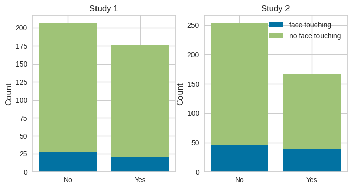
Example 2: Mask-wearing and face-touching#
Figure 17.8#
maskdata = pd.read_csv('https://raw.githubusercontent.com/statsthinking21/statsthinking21-figures-data/main/mask_wearing/DataVersion2/MaskFaceTouchOSF.csv')
maskdata = maskdata.query('face_touching != "Missing"')
maskdata.face_touching = np.where(maskdata.face_touching == 'Yes', 1, 0)
maskdata.mask_front_touching = np.where(maskdata.mask_front_touching == 'Yes', 1, 0)
maskdata.mask_strap_touching = np.where(maskdata.mask_strap_touching == 'Yes', 1, 0)
maskdata['face_touching'] = np.clip(maskdata.face_touching + maskdata.mask_front_touching + maskdata.mask_strap_touching, None, 1)
maskdata['mask_wearing'] = np.where(maskdata.mask_YesNo == 'Yes', 1, 0)
maskdata['age_std'] = scale(maskdata.age)
maskdata['segment_crowding_std'] = scale(maskdata.segment_crowding)
maskdata = maskdata.query('change == 0 and non_covering != "Yes"')

maskdata_study1 = maskdata.query('study == 1')
maskdata_study2 = maskdata.query('study == 2')
# there is no built-in stacked bar plot function in seaborn

fig, ax = plt.subplots(1, 2, figsize=(8,4))

study1_sums = maskdata_study1.groupby('mask_wearing')['face_touching'].value_counts()
study2_sums = maskdata_study2.groupby('mask_wearing')['face_touching'].value_counts()

labels = ['No', 'Yes']
ax[0].bar(labels, study1_sums.loc[:, 1], label='face touching')
ax[0].bar(labels, study1_sums.loc[:, 0], bottom=study1_sums.loc[:, 1], label='no face touching')

ax[1].bar(labels, study2_sums.loc[:, 1], label='face touching')
ax[1].bar(labels, study2_sums.loc[:, 0], bottom=study2_sums.loc[:, 1], label='no face touching')
ax[1].legend()

for i in range(2):
    ax[i].set_ylabel('Count')
    ax[i].set_title(f'Study {i + 1}')

plt.show()
simple chi-squared test
pg.chi2_independence(maskdata_study1, 'mask_wearing', 'face_touching')[2].loc[0, :]
test       pearson
lambda         1.0
chi2      0.029801
dof            1.0
pval      0.862943
cramer    0.008821
power     0.053421
Name: 0, dtype: object
analogous test for the data from the second study
pg.chi2_independence(maskdata_study2, 'mask_wearing', 'face_touching')[2].loc[0, :]
test       pearson
lambda         1.0
chi2      1.085429
dof            1.0
pval      0.297486
cramer    0.050776
power     0.180619
Name: 0, dtype: object
Logistic regression model including duration and study along with mask wearing
glm_mask1 = smf.glm(
    formula='face_touching ~ mask_wearing + duration_of_observation + study',
    data=maskdata,
    family=sm.families.Binomial())
logistic_result_mask1 = glm_mask1.fit()

print(logistic_result_mask1.summary())
                 Generalized Linear Model Regression Results
==============================================================================
Dep. Variable:          face_touching   No. Observations:                  804
Model:                            GLM   Df Residuals:                      800
Model Family:                Binomial   Df Model:                            3
Link Function:                  Logit   Scale:                          1.0000
Method:                          IRLS   Log-Likelihood:                -342.50
Date:                Tue, 21 Feb 2023   Deviance:                       685.00
Time:                        21:53:28   Pearson chi2:                     806.
No. Iterations:                     5   Pseudo R-squ. (CS):            0.04025
Covariance Type:            nonrobust
===========================================================================================
                              coef    std err          z      P>|z|      [0.025      0.975]
-------------------------------------------------------------------------------------------
Intercept                  -3.3426      0.392     -8.538      0.000      -4.110      -2.575
mask_wearing                0.1919      0.198      0.970      0.332      -0.196       0.579
duration_of_observation     0.0290      0.006      4.689      0.000       0.017       0.041
study                       0.5717      0.200      2.852      0.004       0.179       0.965
===========================================================================================
# clean up maskdata for use within R

maskdata = maskdata[['face_touching', 'mask_wearing', 'duration_of_observation', 'study', 'unique_situation']]
%%R -i maskdata

glm_result_combined = glm(face_touching ~ mask_wearing + duration_of_observation + study,
                          family=binomial, data=maskdata)
print(summary(glm_result_combined))
Call:
glm(formula = face_touching ~ mask_wearing + duration_of_observation +
    study, family = binomial, data = maskdata)
Deviance Residuals:
Min
1Q
Median
3Q
Max
-1.7465
-0.6011
-0.5299
-0.4732
2.1918
Coefficients:
Estimate
Std. Error
z value
Pr(>|z|)
(Intercept)
-3.342553
0.391507
-8.538
< 2e-16
***
mask_wearing
0.191901
0.197742
0.970
0.33182
duration_of_observation
0.028991
0.006182
4.689
2.74e-06
***
study
0.571684
0.200441
2.852
0.00434
**
---
Signif. codes:
0 ‘***’ 0.001 ‘**’ 0.01 ‘*’ 0.05 ‘.’ 0.1 ‘ ’ 1
(Dispersion parameter for
binomial
family taken to be
1
)
Null deviance: 718.03 on 803 degrees of freedom
Residual deviance: 685.00 on 800 degrees of freedom
AIC:
693
Number of Fisher Scoring iterations:
4
Mixed effects model#
There is no exact replica of glmer() within Python. The statsmodels package includes a function for estimating the parameters of a mixed effect logistic regression model using Bayesian estimation, which we show here for comparison.
random = {"a": '0 + C(unique_situation)', "b": '0 + C(unique_situation) * mask_wearing'}
glm_result = BinomialBayesMixedGLM.from_formula('face_touching ~ mask_wearing + duration_of_observation', random, maskdata)

fitted_glm_result = glm_result.fit_vb()
print(fitted_glm_result.summary())
                      Binomial Mixed GLM Results
======================================================================
                        Type Post. Mean Post. SD   SD  SD (LB) SD (UB)
----------------------------------------------------------------------
Intercept                  M    -2.5007   0.0980
mask_wearing               M     0.1138   0.1473
duration_of_observation    M     0.0293   0.0032
a                          V    -1.0124   0.0624 0.363   0.321   0.412
b                          V    -1.5560   0.0441 0.211   0.193   0.230
======================================================================
Parameter types are mean structure (M) and variance structure (V)
Variance parameters are modeled as log standard deviations
/opt/conda/lib/python3.10/site-packages/statsmodels/genmod/bayes_mixed_glm.py:793: UserWarning: VB fitting did not converge
  warnings.warn("VB fitting did not converge")
This function doesn’t give p-values, but we can compute the probability that each of the parameters is greater than zero, using the mean and standard deviation estimates.
p_mask_wearing = 1- norm.cdf(0, loc=-fitted_glm_result.fe_mean[1], scale=fitted_glm_result.fe_sd[1])
p_duration = 1 - norm.cdf(0, loc=-fitted_glm_result.fe_mean[2], scale=fitted_glm_result.fe_sd[2])

print('P(mask_wearing <= 0| data) =', p_mask_wearing)
print('P(duration <= 0| data) =', p_duration)
P(mask_wearing <= 0| data) = 0.21993044746773704
P(duration <= 0| data) = 0.0
Compute in R for comparison
%%R -i maskdata
library(lme4)
library(tidyverse)
glmer_result = glmer(face_touching ~ mask_wearing + duration_of_observation + (1 + mask_wearing  |unique_situation), data=maskdata, family=binomial)
glmer_result_baseline = update(glmer_result, formula = ~ . -mask_wearing)  # Without mask effect term

maskdata = maskdata %>%
  mutate(glmer_resid = residuals(glmer_result),
         )

print(summary(glmer_result))
Generalized linear mixed model fit by maximum likelihood (Laplace
Approximation)
[
glmerMod
]
Family:
binomial
( logit )
Formula:
face_touching ~ mask_wearing + duration_of_observation + (1 +
mask_wearing | unique_situation)
Data:
maskdata
AIC
BIC
logLik
deviance
df.resid
704.2
732.4
-346.1
692.2
798
Scaled residuals:
Min
1Q
Median
3Q
Max
-1.6847
-0.4289
-0.3888
-0.3335
3.1095
Random effects:
Groups
Name
Variance
Std.Dev.
Corr
unique_situation
(Intercept)
0.1829
0.4277
mask_wearing
0.1599
0.3999
-0.40
Number of obs: 804, groups:
unique_situation, 129
Fixed effects:
Estimate
Std. Error
z value
Pr(>|z|)
(Intercept)
-2.518255
0.245319
-10.265
< 2e-16
***
mask_wearing
0.145705
0.253822
0.574
0.566
duration_of_observation
0.029691
0.006409
4.633
3.61e-06
***
---
Signif. codes:
0 ‘***’ 0.001 ‘**’ 0.01 ‘*’ 0.05 ‘.’ 0.1 ‘ ’ 1
Correlation of Fixed Effects:
(Intr)
msk_wr
mask_wearng
-0.471
drtn_f_bsrv
-0.698
-0.011
test for overdispersion:
%%R

print(testDispersion(glmer_result, alternative='greater', type='PearsonChisq'))
Parametric dispersion test via mean Pearson-chisq statistic
data:
glmer_result
dispersion = 0.92427, df = 798, p-value = 0.9377
alternative hypothesis:
greater
Figure 17.9#
We do this in R since otherwise we would have to work with the glmer result in Python, which is difficult.
%%R

library(broom.mixed)
library(psych)
loess_logit_est2 = function(iv, span=1){
  fit = loess(face_touching_int ~ iv, data=maskmodeldata, span=span)$fitted
  fit[fit<=0] = 0 #negatives can happen at edges
  logit_of_fit = logit(fit)
  return(logit_of_fit)
}


maskmodeldata = augment(glmer_result) %>%
  mutate(face_touching_int = as.integer(face_touching))
maskmodeldata = maskmodeldata %>%
  mutate(observed_logit = loess_logit_est2(duration_of_observation))

ggplot(maskmodeldata, aes(duration_of_observation, observed_logit, size=.cooksd))+
  geom_jitter() +
  geom_smooth(method = "loess", se=FALSE)
R[write to console]:
Attaching package: ‘psych’
R[write to console]: The following objects are masked from ‘package:ggplot2’:

    %+%, alpha
`geom_smooth()` using formula = 'y ~ x'
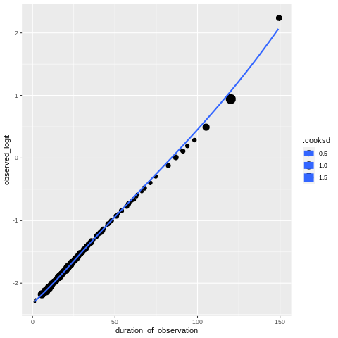
Table 17.3#
here too we use R code
%%R

effect_table = tidy(glmer_result,conf.int=TRUE,exponentiate=TRUE,effects="fixed") %>%
  dplyr::select(term, estimate, conf.low, conf.high)

names(effect_table) = c('', 'Odds ratio', '2.5 %', '97.5 %')
effect_table[2:3,]
# A tibble: 2 × 4
`` `Odds ratio` `2.5 %` `97.5 %`
<chr> <dbl> <dbl> <dbl>
1 mask_wearing 1.16 0.703 1.90
2 duration_of_observation 1.03 1.02 1.04
Example 3: Asthma and air pollution#
3. Prepare the data for analysis#
pmdata = pd.read_csv('https://raw.githubusercontent.com/statsthinking21/statsthinking21-figures-data/main/CDC_PM2.5_2014/Daily_Census_Tract-Level_PM2.5_mean_2014.csv').rename(
    columns={'ctfips': 'TractFIPS', 'ds_pm_pred': 'pm25_mean'})

asthmadata = pd.read_csv('https://raw.githubusercontent.com/statsthinking21/statsthinking21-figures-data/main/500cities_disease/acsdata_with_censusdata.csv')
asthmadata.set_index('TractFIPS', inplace=True)

asthmadata.drop([i for i in asthmadata.columns if '_Crude95CI' in i], axis=1, inplace=True)

pm_asthma_data = pmdata.join(asthmadata, how='inner', on='TractFIPS', rsuffix='_r').dropna().rename(
    columns={'CASTHMA_CrudePrev': 'asthma_prev', 'PlaceFIPS': 'city'})
pm_asthma_data.MedianIncome = pm_asthma_data.MedianIncome / 1000
pm_asthma_data.Population2010 = pm_asthma_data.Population2010 / 1000
pm_asthma_data.reset_index(inplace=True)
%%R

# asthma data
# https://chronicdata.cdc.gov/500-Cities-Places/500-Cities-Census-Tract-level-Data-GIS-Friendly-Fo/5mtz-k78d (for 2014)
#
# PM2.5 data:
#
# filtered for 2014 and averaged ds_pm_pred using:
#
# https://data.cdc.gov/Environmental-Health-Toxicology/Daily-Census-Tract-Level-PM2-5-Concentrations-2011/fcqm-xrf4/data


pmdata = read_csv('https://raw.githubusercontent.com/statsthinking21/statsthinking21-figures-data/main/CDC_PM2.5_2014/Daily_Census_Tract-Level_PM2.5_mean_2014.csv') %>%
  rename(TractFIPS=ctfips,
         pm25_mean=ds_pm_pred)

asthmadata = read_csv('https://raw.githubusercontent.com/statsthinking21/statsthinking21-figures-data/main/500cities_disease/acsdata_with_censusdata.csv') %>%
  dplyr::select(-ends_with('_Crude95CI'))

pm_asthma_data = inner_join(asthmadata, pmdata, by='TractFIPS') %>%
  drop_na() %>%
  rename(asthma_prev=CASTHMA_CrudePrev,
         city=PlaceFIPS) %>%
  mutate(MedianIncome = MedianIncome/1000,
         Population2010 = Population2010/1000)
  # mutate(log_asthma_prev = log(asthma_prev))

dim(pm_asthma_data)
Rows: 72283 Columns: 2
── Column specification ────────────────────────────────────────────────────────
Delimiter: ","
dbl (2): ctfips, ds_pm_pred
ℹ Use `spec()` to retrieve the full column specification for this data.
ℹ Specify the column types or set `show_col_types = FALSE` to quiet this message.
Rows: 26892 Columns: 66
── Column specification ────────────────────────────────────────────────────────
Delimiter: ","
chr (33): StateAbbr, PlaceName, Place_TractID, ACCESS2_Crude95CI, ARTHRITIS_...
dbl (33): PlaceFIPS, TractFIPS, Population2010, ACCESS2_CrudePrev, ARTHRITIS...
ℹ Use `spec()` to retrieve the full column specification for this data.
ℹ Specify the column types or set `show_col_types = FALSE` to quiet this message.
[1]
26681
39
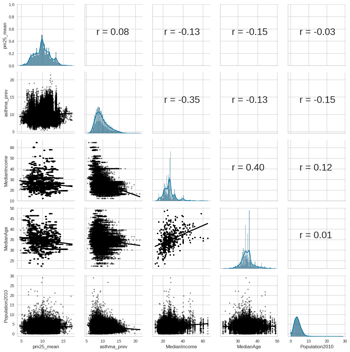
Figure 17.10#
plt.figure(figsize=(12,12))
g = sns.PairGrid(pm_asthma_data[['pm25_mean', 'asthma_prev', 'MedianIncome', 'MedianAge', 'Population2010']])

def corrfunc(x, y, hue=None, ax=None, **kws):
    """Plot the correlation coefficient in the top left hand corner of a plot."""
    r, _ = pearsonr(x, y)
    ax = ax or plt.gca()
    ax.annotate(f'r = {r:.2f}', xy=(.2, .5), size=24, xycoords=ax.transAxes)

g.map_upper(corrfunc)
g.map_lower(sns.regplot, color='black', scatter_kws={'s': 10, 'alpha':.5})
g.map_diag(sns.histplot, kde=True, legend=False)
plt.show()
<Figure size 1200x1200 with 0 Axes>
standard linear regression model
lm_asthma_pm = smf.ols('asthma_prev ~ pm25_mean + MedianIncome +  MedianAge + Population2010', data=pm_asthma_data).fit()
print(lm_asthma_pm.summary())
                            OLS Regression Results
==============================================================================
Dep. Variable:            asthma_prev   R-squared:                       0.137
Model:                            OLS   Adj. R-squared:                  0.137
Method:                 Least Squares   F-statistic:                     1061.
Date:                Tue, 21 Feb 2023   Prob (F-statistic):               0.00
Time:                        21:54:14   Log-Likelihood:                -54500.
No. Observations:               26681   AIC:                         1.090e+05
Df Residuals:                   26676   BIC:                         1.091e+05
Df Model:                           4
Covariance Type:            nonrobust
==================================================================================
                     coef    std err          t      P>|t|      [0.025      0.975]
----------------------------------------------------------------------------------
Intercept         12.5516      0.150     83.796      0.000      12.258      12.845
pm25_mean          0.0328      0.006      5.294      0.000       0.021       0.045
MedianIncome      -0.1096      0.002    -53.969      0.000      -0.114      -0.106
MedianAge          0.0047      0.004      1.202      0.229      -0.003       0.012
Population2010    -0.1136      0.006    -19.105      0.000      -0.125      -0.102
==============================================================================
Omnibus:                     2192.456   Durbin-Watson:                   1.967
Prob(Omnibus):                  0.000   Jarque-Bera (JB):             2804.084
Skew:                           0.741   Prob(JB):                         0.00
Kurtosis:                       3.569   Cond. No.                         592.
==============================================================================

Notes:
[1] Standard Errors assume that the covariance matrix of the errors is correctly specified.
Figure 17.11#
model_data = pd.DataFrame({'resid': lm_asthma_pm.resid}, index=pm_asthma_data.index)
fig = sm.qqplot(model_data.resid, line="q")
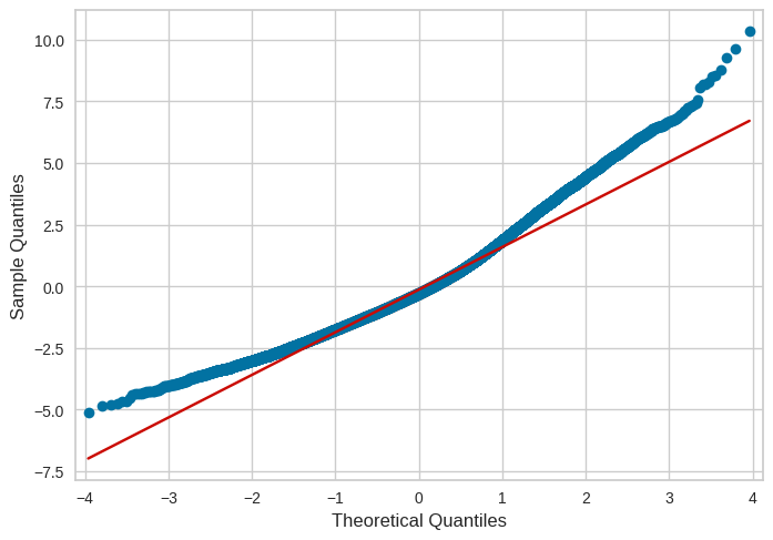
Figure 17.12#
# first fit linear mixed effects model

lme = smf.mixedlm("asthma_prev ~ pm25_mean + MedianAge + MedianIncome + Population2010",
                  pm_asthma_data, groups=pm_asthma_data["city"],
                re_formula="~pm25_mean").fit(method=["lbfgs"])
print(lme.summary())
              Mixed Linear Model Regression Results
=================================================================
Model:                MixedLM   Dependent Variable:   asthma_prev
No. Observations:     26681     Method:               REML
No. Groups:           494       Scale:                1.9514
Min. group size:      8         Log-Likelihood:       -48031.9272
Max. group size:      2110      Converged:            Yes
Mean group size:      54.0
-----------------------------------------------------------------
                       Coef.  Std.Err.   z    P>|z| [0.025 0.975]
-----------------------------------------------------------------
Intercept               6.977    1.146  6.087 0.000  4.730  9.223
pm25_mean               0.360    0.074  4.856 0.000  0.215  0.506
MedianAge               0.050    0.028  1.754 0.079 -0.006  0.105
MedianIncome           -0.103    0.014 -7.125 0.000 -0.132 -0.075
Population2010         -0.027    0.005 -5.652 0.000 -0.037 -0.018
Group Var             158.916   15.957
Group x pm25_mean Cov -15.097    1.536
pm25_mean Var           1.458    0.150
=================================================================
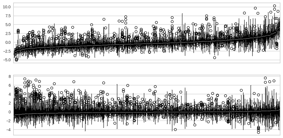
model_data['city'] = pm_asthma_data.city
model_data['resid_lme'] = lme.resid

def boxplot_sorted(df, by, column, ax):
    df2 = pd.DataFrame({col:vals[column] for col, vals in df.groupby(by)})
    meds = df2.median().sort_values()
    plot = df2[meds.index].boxplot(rot=90, ax=ax)
    plot.get_xaxis().set_ticks([])

fig, ax = plt.subplots(2, 1, figsize=(12,6))

boxplot_sorted(model_data, 'city', 'resid', ax=ax[0])

boxplot_sorted(model_data, 'city', 'resid_lme', ax=ax[1])
R mixed effect model result for comparison
%%R
library(lme4)
lmer_asthma_pm = lmer(asthma_prev ~ pm25_mean + MedianAge + MedianIncome + Population2010 + (1 + pm25_mean|city),
                    data=pm_asthma_data,
                     control = lmerControl(
                           optimizer ='optimx', optCtrl=list(method='nlminb')))
print(summary(lmer_asthma_pm))
R[write to console]: Loading required namespace: optimx
Linear mixed model fit by REML ['lmerMod']
Formula:
asthma_prev ~ pm25_mean + MedianAge + MedianIncome + Population2010 +
(1 + pm25_mean | city)
Data:
pm_asthma_data
Control:
lmerControl(optimizer = "optimx", optCtrl = list(method = "nlminb"))
REML criterion at convergence:
96063.9
Scaled residuals:
Min
1Q
Median
3Q
Max
-3.3329
-0.6246
-0.0829
0.5462
5.4814
Random effects:
Groups
Name
Variance
Std.Dev.
Corr
city
(Intercept)
158.898
12.605
pm25_mean
1.457
1.207
-0.99
Residual
1.951
1.397
Number of obs: 26681, groups:
city, 494
Fixed effects:
Estimate
Std. Error
t value
(Intercept)
6.976828
1.122358
6.216
pm25_mean
0.360445
0.071826
5.018
MedianAge
0.049659
0.028236
1.759
MedianIncome
-0.103198
0.014298
-7.217
Population2010
-0.027124
0.004796
-5.655
Correlation of Fixed Effects:
(Intr)
pm25_m
MednAg
MdnInc
pm25_mean
-0.646
MedianAge
-0.698
0.002
MedianIncom
0.098
-0.005
-0.506
Popultn2010
-0.017
-0.006
0.010
-0.016
optimizer (optimx) convergence code: 0 (OK)
Model failed to converge with max|grad| = 0.00298875 (tol = 0.002, component 1)
Table 17.4#
lme_ci = pd.DataFrame(lme.params, columns=['estimate'])
lme_ci = lme_ci.join(lme.conf_int().rename(columns={0: '2.5%', 1:'97.5%'})).iloc[1:5,:]
lme_ci
| estimate | 2.5% | 97.5% | |
|---|---|---|---|
| pm25_mean | 0.360453 | 0.214966 | 0.505941 |
| MedianAge | 0.049660 | -0.005829 | 0.105149 |
| MedianIncome | -0.103198 | -0.131586 | -0.074811 |
| Population2010 | -0.027124 | -0.036531 | -0.017718 |
Example 4: Response of plants to nitrogen fertilizers and soil tilling#
3. Prepare and visualize the data#
fert_data_all = pd.read_csv('https://raw.githubusercontent.com/statsthinking21/statsthinking21-figures-data/main/fertilizer/Fertsyntraitsall_Jan27_2008.txt', delimiter='\t')
fert_data_all = fert_data_all.query('Rawabundmetric == "Grams biomass" and Site == "KBS"')
fert_data_all['plotID_common'] = fert_data_all.plotID = fert_data_all.Fert
fert_data_all['log_rawabund'] = scale(np.log(fert_data_all.Rawabund))

fert_data_all.shape
(2615, 27)
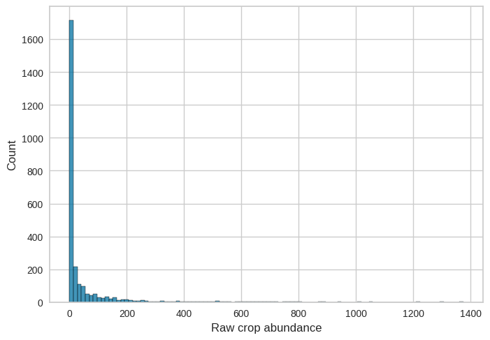
Figure 17.13#
sns.histplot(fert_data_all.Rawabund, bins=100)
plt.xlabel('Raw crop abundance')
Text(0.5, 0, 'Raw crop abundance')
Simple linear model output:
lm_result_fert = smf.ols('Rawabund ~ Fert*Experiment + Year', data=fert_data_all).fit()
print(lm_result_fert.summary())
                            OLS Regression Results
==============================================================================
Dep. Variable:               Rawabund   R-squared:                       0.030
Model:                            OLS   Adj. R-squared:                  0.029
Method:                 Least Squares   F-statistic:                     20.52
Date:                Tue, 21 Feb 2023   Prob (F-statistic):           1.16e-16
Time:                        21:54:43   Log-Likelihood:                -16314.
No. Observations:                2615   AIC:                         3.264e+04
Df Residuals:                    2610   BIC:                         3.267e+04
Df Model:                           4
Covariance Type:            nonrobust
===============================================================================================
                                  coef    std err          t      P>|t|      [0.025      0.975]
-----------------------------------------------------------------------------------------------
Intercept                    1154.5206   1685.230      0.685      0.493   -2150.002    4459.043
Experiment[T.Untilled]         -5.3171      6.568     -0.810      0.418     -18.196       7.562
Fert                           57.1985      7.608      7.518      0.000      42.280      72.117
Fert:Experiment[T.Untilled]   -35.4946      9.933     -3.573      0.000     -54.972     -16.018
Year                           -0.5602      0.844     -0.664      0.507      -2.215       1.094
==============================================================================
Omnibus:                     2428.192   Durbin-Watson:                   1.041
Prob(Omnibus):                  0.000   Jarque-Bera (JB):            84679.507
Skew:                           4.496   Prob(JB):                         0.00
Kurtosis:                      29.388   Cond. No.                     1.39e+06
==============================================================================

Notes:
[1] Standard Errors assume that the covariance matrix of the errors is correctly specified.
[2] The condition number is large, 1.39e+06. This might indicate that there are
strong multicollinearity or other numerical problems.
Figure 17.14#
This figure involves fitting a linear mixed model with multiple random slopes. This is in theory possible using statsmodels, but it is not well documented. Instead, we will simply use the R bridge to run lmer on our data.
fert_data_clean = fert_data_all[['log_rawabund', 'Fert', 'Experiment', 'Year', 'plotID_common', 'Species_code']]
%%R -i fert_data_clean

lm.result_fert = lm(log_rawabund ~ Fert*Experiment + Year ,
                        data=fert_data_clean)

lmer.result_fert = lmer(log_rawabund ~ Fert*Experiment + Year + (1 + Fert|plotID_common) + (1 + Fert|Species_code) ,
                        data=fert_data_clean)
%%R

library(cowplot)
library(broom)
model.data = augment(lm.result_fert) %>%
  mutate(plotID_common = fert_data_clean$plotID_common,
         Species_code = fert_data_clean$Species_code)

p1 = ggplot(model.data, aes(sample=.resid)) + geom_qq() + geom_qq_line()

lmer.result_fert = lmer(log_rawabund ~ Fert*Experiment + Year + (1 + Fert|plotID_common) + (1 + Fert|Species_code),
                        data=fert_data_clean)

fert_data = fert_data_clean %>%
  mutate(lmer_resid = resid(lmer.result_fert))

p2 = ggplot(fert_data, aes(sample=lmer_resid)) + geom_qq() + geom_qq_line()
plot_grid(p1, p2)
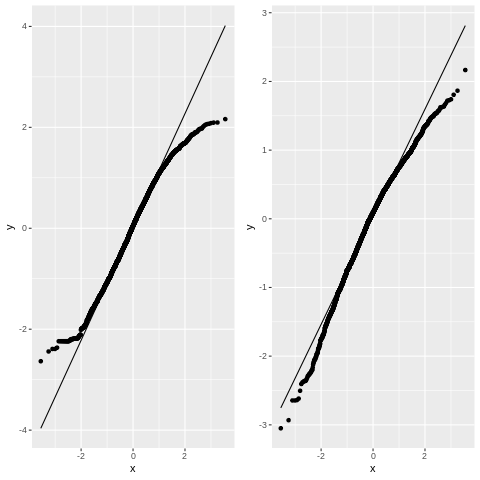
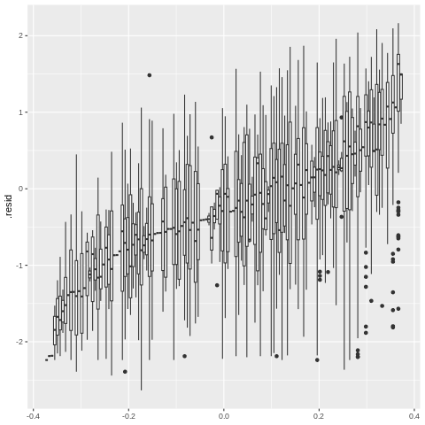
Figure 17.15#
%%R

model_means_sorted = model.data %>% group_by(Species_code) %>%
  summarize_all(mean) %>%
  arrange(.resid)
ggplot(model.data, aes(y=.resid, group=factor(Species_code, levels=model_means_sorted$Species_code))) + geom_boxplot()
Linear mixed effects model output:
%%R

print(summary(lmer.result_fert))
Linear mixed model fit by REML ['lmerMod']
Formula:
log_rawabund ~ Fert * Experiment + Year + (1 + Fert | plotID_common) +
(1 + Fert | Species_code)
Data:
fert_data_clean
REML criterion at convergence:
6476.4
Scaled residuals:
Min
1Q
Median
3Q
Max
-3.8583
-0.6309
0.1140
0.7059
2.7394
Random effects:
Groups
Name
Variance
Std.Dev.
Corr
Species_code
(Intercept)
0.32074
0.5663
Fert
0.07087
0.2662
0.01
plotID_common
(Intercept)
0.64447
0.8028
Fert
0.48111
0.6936
0.31
Residual
0.62516
0.7907
Number of obs: 2615, groups:
Species_code, 132; plotID_common, 2
Fixed effects:
Estimate
Std. Error
t value
(Intercept)
13.420304
11.377770
1.180
Fert
0.279636
1.454441
0.192
ExperimentUntilled
0.384860
0.057878
6.649
Year
-0.006994
0.005681
-1.231
Fert:ExperimentUntilled
-0.333301
0.081763
-4.076
Correlation of Fixed Effects:
(Intr)
Fert
ExprmU
Year
Fert
-0.039
ExprmntUntl
-0.083
0.016
Year
-0.997
0.000
0.080
Frt:ExprmnU
-0.008
-0.036
-0.522
0.010
optimizer (nloptwrap) convergence code: 0 (OK)
unable to evaluate scaled gradient
Model failed to converge: degenerate Hessian with 2 negative eigenvalues
Effect sizes
%%R

library(emmeans)
emm = emmeans(lmer.result_fert, pairwise ~ Fert*Experiment)
print(contrast(emm, 'tukey'))
contrast
estimate
SE
df
t.ratio
p.value
Fert0 Tilled - Fert1 Tilled
-0.2796
1.4545
15559535
-0.192
0.9975
Fert0 Tilled - Fert0 Untilled
-0.3849
0.0583
1183
-6.597
<.0001
Fert0 Tilled - Fert1 Untilled
-0.3312
1.4542
41417709
-0.228
0.9958
Fert1 Tilled - Fert0 Untilled
-0.1052
1.4547
29073394
-0.072
0.9999
Fert1 Tilled - Fert1 Untilled
-0.0516
0.0722
759
-0.714
0.8914
Fert0 Untilled - Fert1 Untilled
0.0537
1.4539
38437869
0.037
1.0000
Degrees-of-freedom method: kenward-roger
P value adjustment: tukey method for comparing a family of 4 estimates